Midterm Study Guide

Note

Answers are here.

Our midterm exam will take place during lecture on Thursday October 8. Here’s what you should know about it:

What’s the format? It’s a traditional pencil-and-paper exam. The questions will be a mix of multiple choice and free response;
How long will it take? You have 75 minutes to complete the exam, but on average the exam is not intended to take the full 75 minutes;
What resources are allowed? You are only allowed both sides of a single 8.5” x 11” sheet of notes created by you and you only. I do not care how you create the note sheet;
Will we be writing code on the exam? No. However, you may be asked to analyze and interpret the output of some code, and so being able to read the code that generated the output could be helpful;
What skills will be emphasized? I care most about your visual intuition and conceptual understanding, so you should sweep through all of the lectures, find every picture we ever dissected, and make sure you understand every detail of it;
What topics will be covered? Everything from Lecture 2 on 9/1 through ~~Lecture 11 on 10/6~~ Lecture 10 on 10/1 is fair game. So that’s exploratory data analysis (visualization and summarization) and regression modeling (both linear and logistic);
Should I study the textbook, the lecture videos, or the tutorials? Maybe if you have time, but you should not prioritize them. In approximate order of importance, you should prioritize studying this guide, the lecture notes, the solutions to the in-class demos (so-called AEs), the homeworks, and the labs. If you have more time to study after all of that, then the first thing I would suggest is sampling some of the odd-numbered exercises at the end of Ch. 1 - 10 in IMS. The answers to these exercises are in the book, and they do not involve code: just concepts, interpretation, etc;
- Note: if you do dip into the textbook, videos, or tutorials, and you encounter a topic that never appeared in any of the lectures, labs, or homeworks, then you are not responsible for it;
One more thing: don’t waste your time studying the details of any specific applications or datasets we’ve seen (eg. penguins, Bechdel, gerrymandering, diamonds, etc). Real datasets will of course be discussed on the exam, but everything you need to know about them will be introduced from scratch within the exam as if you had never seen them before.

Below are a bunch of practice problems to get your wheels spinning. Solutions will be posted on Monday October 5.

Try this

Attempt all of the problems below without resources. Make note of your pain points and blind spots along the way. That might give you an idea of the stuff you would benefit from if you had it on a cheat sheet.

Concepts and main ideas

Question 1

Can you answer each of these in one or two sentences?

If I have a column of numbers, what is the definition of the 38% quantile?
- Could you sketch a cartoon of what this looks like?
- Is the 38% quantile smaller than, bigger than, or equal to the median, or do you not have enough information to say?
What does the correlation coefficient between two numerical variables measure?
What is the difference between $y=\beta_0+\beta_1 x + \varepsilon$ and $\hat{y}=b_0+b_1 x$?
When we plot a line of best fit for a numerical predictor and numerical response, what does “best” mean?
Consider this bit of toy code: linear_reg() |> fit(_BLANK_, df)? What goes in the blank? What purpose does that argument serve, and how do you use it?
Under what circumstances is the intercept in a regression model a meaningful quantity?
If you run a “simple” linear regression model with a numerical response and a categorical predictor with three levels, what does the computer actually do to estimate that model?
Let $\hat{y}^{(\text{old})}$ be the prediction at $x$ of a simple linear regression, and let $\hat{y}^{(\text{new})}$ be the prediction at $x+1$ of the same regression. How are $\hat{y}^{(\text{old})}$ and $\hat{y}^{(\text{new})}$ related? In other words, how does the prediction of the simple linear regression model change when you change the input from $x$ to $x+1$?
What does the $R^2$ of a linear regression measure?
Why is adjusted $R^2$ a better model selection criterion than ordinary, unadjusted $R^2$?
Let $\hat{o}^{(\text{old})}$ be the estimated odds at $x$ from a simple logistic regression model, and let $\hat{o}^{(\text{new})}$ be the estimated odds at $x+1$ of the same regression. How are $\hat{o}^{(\text{old})}$ and $\hat{o}^{(\text{new})}$ related? In other words, how does the prediction of the simple logistic regression model change when you change the input from $x$ to $x+1$?
What is the main lesson of Anscombe’s Quartet?

Visual understanding

Question 2

Practice!

https://www.rossmanchance.com/applets/2021/guesscorrelation/GuessCorrelation.html

Question 3

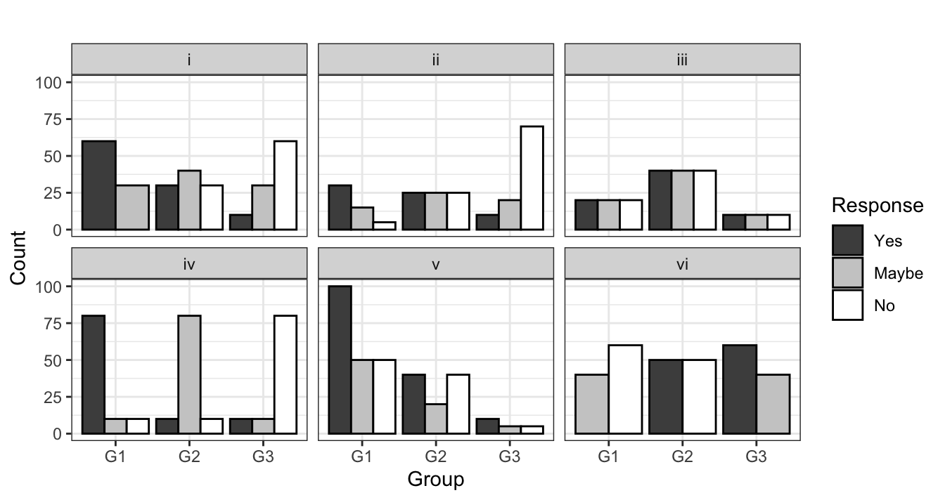
Match the “dodged” barchart with the corresponding stacked barchart. There is exactly one unique match for each.

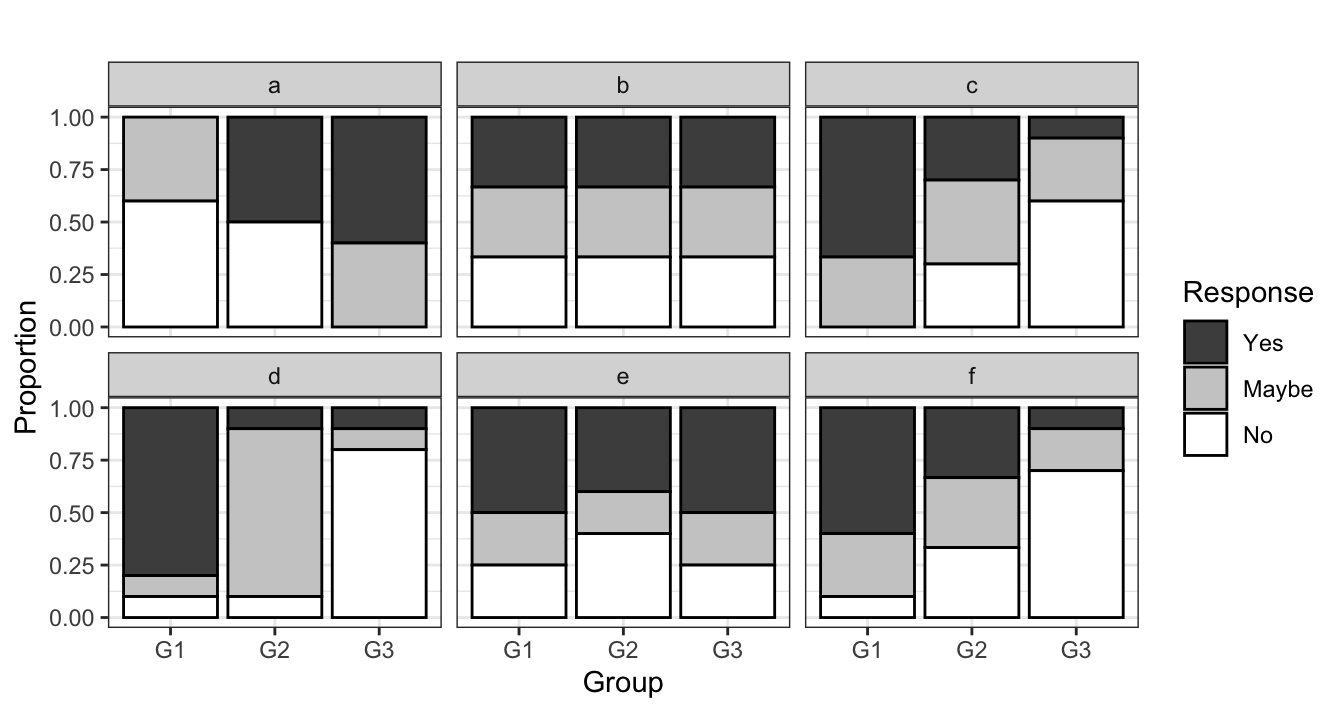
Question 4

The scatterplots below show the relationships between six pairs of x and y variables.

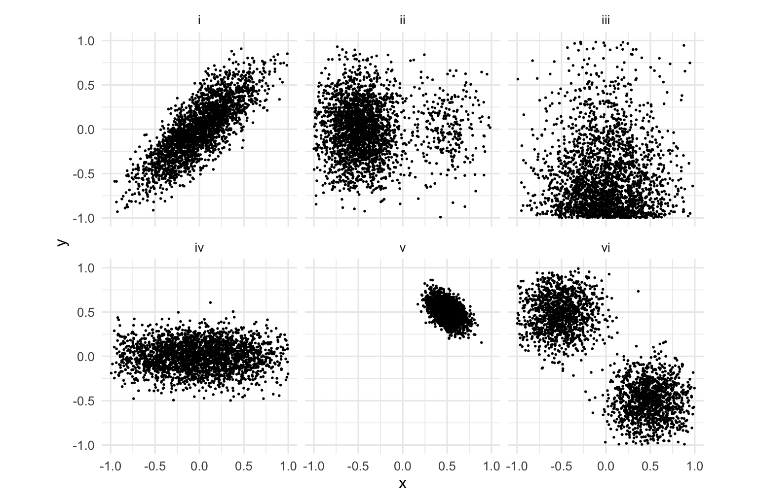
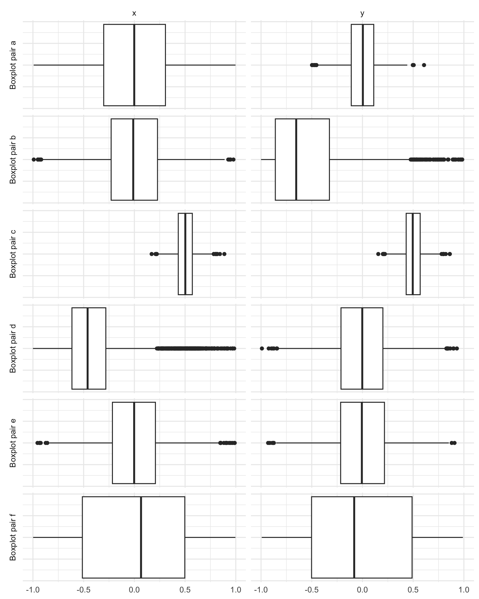
Match each scatterplot to the pair of boxplots that displays the distributions of x and y separately. There is exactly one unique match for each.

Hint

Notice that the range of the axes is the same in every picture.

Question 5

In what follows, let $y$ be a binary response, let $x$ be a numerical predictor, and let $z$ be a binary predictor. Match the S-curve to the model equation.

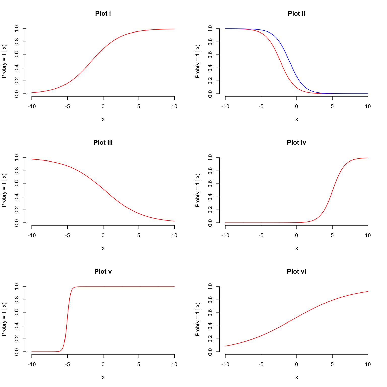
$\log\left(\frac{\hat{p}}{1-\hat{p}}\right) = 22.9 + 4.54 \times x$
$\log\left(\frac{\hat{p}}{1-\hat{p}}\right) = 0.118 + 0.246 \times x$
$\log\left(\frac{\hat{p}}{1-\hat{p}}\right) = 0.798 + 0.486 \times x$
$\log\left(\frac{\hat{p}}{1-\hat{p}}\right) = -6.035 + 1.194 \times x$
$\log\left(\frac{\hat{p}}{1-\hat{p}}\right) = -2.26 - 0.99 \times x+1.26\times z$
$\log\left(\frac{\hat{p}}{1-\hat{p}}\right) = 0.079 -0.373 \times x$

STAWANOWA doctor

What’s wrong with the interpretations below? Diagnose the problem and fix it if possible.

Question 6

Some bozo ran this regression and wrote the following interpretation:

linear_reg() |>
  fit(bill_length_mm ~ flipper_length_mm, penguins) |>
  tidy()

# A tibble: 2 × 5
  term              estimate std.error statistic  p.value
  <chr>                <dbl>     <dbl>     <dbl>    <dbl>
1 (Intercept)         -7.26     3.20       -2.27 2.38e- 2
2 flipper_length_mm    0.255    0.0159     16.0  1.74e-43

If the flipper length of a penguin increases by 1mm, then the bill length will increase by 0.25mm.

Question 7

Some schmuck ran this regression and wrote the following interpretation:

logistic_reg() |>
  fit(spam ~ num_char, email) |>
  tidy()

# A tibble: 2 × 5
  term        estimate std.error statistic   p.value
  <chr>          <dbl>     <dbl>     <dbl>     <dbl>
1 (Intercept)  -1.80     0.0716     -25.1  2.04e-139
2 num_char     -0.0621   0.00801     -7.75 9.50e- 15

If the number of characters in an email increases by 1000, then the estimated probability of that email being spam is lower by -0.062, on average.

FYI: from the documentation (?email), num_char is “The number of characters in the email, in thousands.”

Question 8

Some putz ran this regression and wrote the following interpretation:

linear_reg() |>
  fit(body_mass_g ~ flipper_length_mm + bill_length_mm, penguins) |> 
  tidy()

# A tibble: 3 × 5
  term              estimate std.error statistic  p.value
  <chr>                <dbl>     <dbl>     <dbl>    <dbl>
1 (Intercept)       -5737.      308.      -18.6  7.80e-54
2 flipper_length_mm    48.1       2.01     23.9  7.56e-75
3 bill_length_mm        6.05      5.18      1.17 2.44e- 1

If flipper length and bill length both increase by 1mm, then we predict that body mass is lower by 48.14 grams, on average.

Question 9

Some blockhead ran this regression and wrote the following interpretation:

linear_reg() |>
  fit(body_mass_g ~ flipper_length_mm * species, penguins) |>
  tidy()

# A tibble: 6 × 5
  term                               estimate std.error statistic  p.value
  <chr>                                 <dbl>     <dbl>     <dbl>    <dbl>
1 (Intercept)                        -2536.      879.      -2.88  4.19e- 3
2 flipper_length_mm                     32.8       4.63     7.10  7.69e-12
3 speciesChinstrap                    -501.     1523.      -0.329 7.42e- 1
4 speciesGentoo                      -4251.     1427.      -2.98  3.11e- 3
5 flipper_length_mm:speciesChinstrap     1.74      7.86     0.222 8.25e- 1
6 flipper_length_mm:speciesGentoo       21.8       6.94     3.14  1.84e- 3

If the flipper length of a Chinstrap penguin increases by 1mm, then we predict that the body mass is higher by 1.74 grams on average.

Question 10

Some nitwit ran this regression and wrote the following interpretation:

linear_reg() |>
  fit(hp ~ mpg, mtcars) |>
  glance()

# A tibble: 1 × 12
  r.squared adj.r.squared sigma statistic     p.value    df logLik   AIC   BIC
      <dbl>         <dbl> <dbl>     <dbl>       <dbl> <dbl>  <dbl> <dbl> <dbl>
1     0.602         0.589  43.9      45.5 0.000000179     1  -165.  337.  341.
# ℹ 3 more variables: deviance <dbl>, df.residual <int>, nobs <int>

About 60% of the observed variation in miles/gallon is explained by the model.

Question 11

Some chooch ran this regression and wrote the following interpretation:

logistic_reg() |>
  fit(spam ~ exclaim_mess + viagra + dollar, email) |>
  tidy()

# A tibble: 4 × 5
  term         estimate std.error statistic p.value
  <chr>           <dbl>     <dbl>     <dbl>   <dbl>
1 (Intercept)  -2.22      0.0568   -39.1    0      
2 exclaim_mess  0.00189   0.00108    1.75   0.0794 
3 viagra        1.86     40.6        0.0459 0.963  
4 dollar       -0.0656    0.0208    -3.15   0.00165

If an email contains no exclamation marks, no dollar signs, and no mentions of viagra, then the model predicts that the probability of it being spam is $e^{-2.218}\approx 0.10886$.

Question 12

Some nincompoop ran this regression and wrote the following interpretation:

linear_reg() |>
  fit(bill_length_mm ~ bill_depth_mm + sex, penguins) |>
  tidy()

# A tibble: 3 × 5
  term          estimate std.error statistic  p.value
  <chr>            <dbl>     <dbl>     <dbl>    <dbl>
1 (Intercept)      61.0      2.35      26.0  7.39e-82
2 bill_depth_mm    -1.15     0.141     -8.16 7.35e-15
3 sexmale           5.44     0.555      9.81 4.18e-20

If a male penguin has a bill depth of 0mm (sad!), then we expect its bill length to be 60.99mm on average.

Question 13

Some silly goose ran this regression and wrote the following interpretation:

linear_reg() |>
  fit(body_mass_g ~ flipper_length_mm + bill_length_mm, penguins) |>
  glance()

# A tibble: 1 × 12
  r.squared adj.r.squared sigma statistic   p.value    df logLik   AIC   BIC
      <dbl>         <dbl> <dbl>     <dbl>     <dbl> <dbl>  <dbl> <dbl> <dbl>
1     0.760         0.759  394.      537. 9.09e-106     2 -2528. 5063. 5079.
# ℹ 3 more variables: deviance <dbl>, df.residual <int>, nobs <int>

The correlation between body mass, flipper length, and bill length is about $\sqrt{0.76}\approx 0.87$.

Data analysis

Law & Order

You’ve heard of the tidyverse, now let’s visit the Law & Order-verse. Doink doink!¹

Law & Order is a police procedural and legal drama television series that has been running since the 1990s. The Law & Order franchise includes a number of series such as Law & Order, Law & Order: SVU, Law & Order: Criminal Intent, etc.

You will work with data on average ratings for each season of three series from the Law & Order-verse – a subset of the data from the previous questions. Below is a peek at the first ten rows of the Law & Order data.

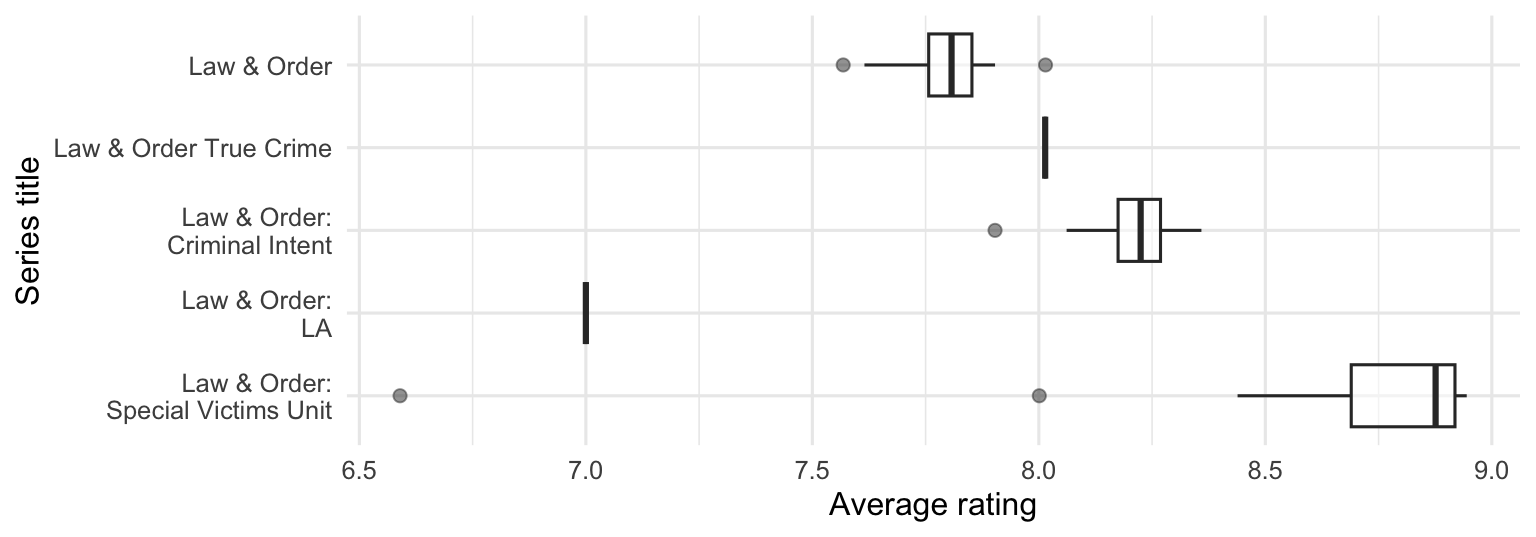
The plot below shows the distributions of average ratings of various Law & Order series across seasons.

Question 14

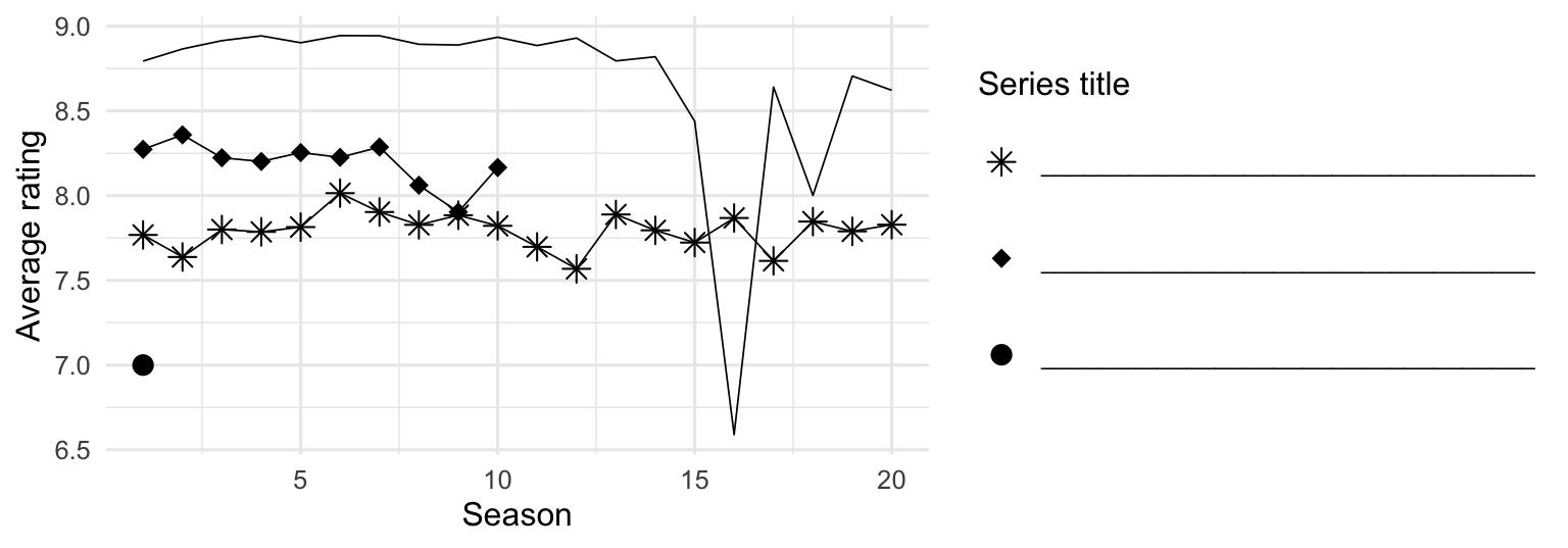
Based on the information from the side-by-side box plots, fill in the legend of the plot below with Law & Order series titles.

Question 15

The following code calculates the standard deviations of average season ratings of the five Law & Order series. Unfortunately, the output is partially erased and replaced with blanks.

lo_titles <- c("Law & Order", "Law & Order: Criminal Intent", "Law & Order: SVU")

law_and_order |>
  filter(title %in% lo_titles) |>
  group_by(title) |>
  summarize(mean_av_rating = mean(av_rating), sd_av_rating = sd(av_rating))

# A tibble: 5 × 3
  title                         mean_av_rating sd_av_rating
  <chr>                                  <dbl>        <dbl>
1 Law & Order                            _(1)_        0.106
2 Law & Order: Criminal Intent            8.20        0.129
4 Law & Order: SVU                        8.67        _(2)_

Based on the visualizations you’ve seen of these data so far, which of the following is true about the blanks in the output? Select all that are true.

The mean of average ratings (Blank 1) of Law & Order seasons is lower than the other two means.
The mean of average ratings (Blank 1) of Law & Order seasons is higher than the other two means.
The standard deviation of average ratings of Law & Order: SVU seasons (Blank 2) is lower than the other two standard deviations.
The standard deviation of average ratings of Law & Order: SVU seasons (Blank 2) is higher than the other two standard deviations.
The standard deviation of average ratings of Law & Order: SVU seasons (Blank 2) is between the other two standard deviations.

Blizzard salaries

In 2020, employees of Blizzard Entertainment circulated a spreadsheet to anonymously share salaries and recent pay increases amidst rising tension in the video game industry over wage disparities and executive compensation. (Source: Blizzard Workers Share Salaries in Revolt Over Pay)

The name of the data frame used for this analysis is blizzard_salary and the variables are:

percent_incr: Raise given in July 2020, as percent increase with values ranging from 1 (1% increase) to 21.5 (21.5% increase)
salary_type: Type of salary, with levels Hourly and Salaried
annual_salary: Annual salary, in USD, with values ranging from $50,939 to $216,856.
performance_rating: Most recent review performance rating, with levels Poor, Successful, High, and Top. The Poor level is the lowest rating and the Top level is the highest rating.

The first ten rows of blizzard_salary are shown below:

# A tibble: 409 × 4
   percent_incr salary_type annual_salary performance_rating
          <dbl> <chr>               <dbl> <chr>             
 1          1   Salaried               1  High              
 2          1   Salaried               1  Successful        
 3          1   Salaried               1  High              
 4          1   Hourly             33987. Successful        
 5         NA   Hourly             34798. High              
 6         NA   Hourly             35360  <NA>              
 7         NA   Hourly             37440  <NA>              
 8          0   Hourly             37814. <NA>              
 9          4   Hourly             41101. Top               
10          1.2 Hourly             42328  <NA>              
# ℹ 399 more rows

Question 16

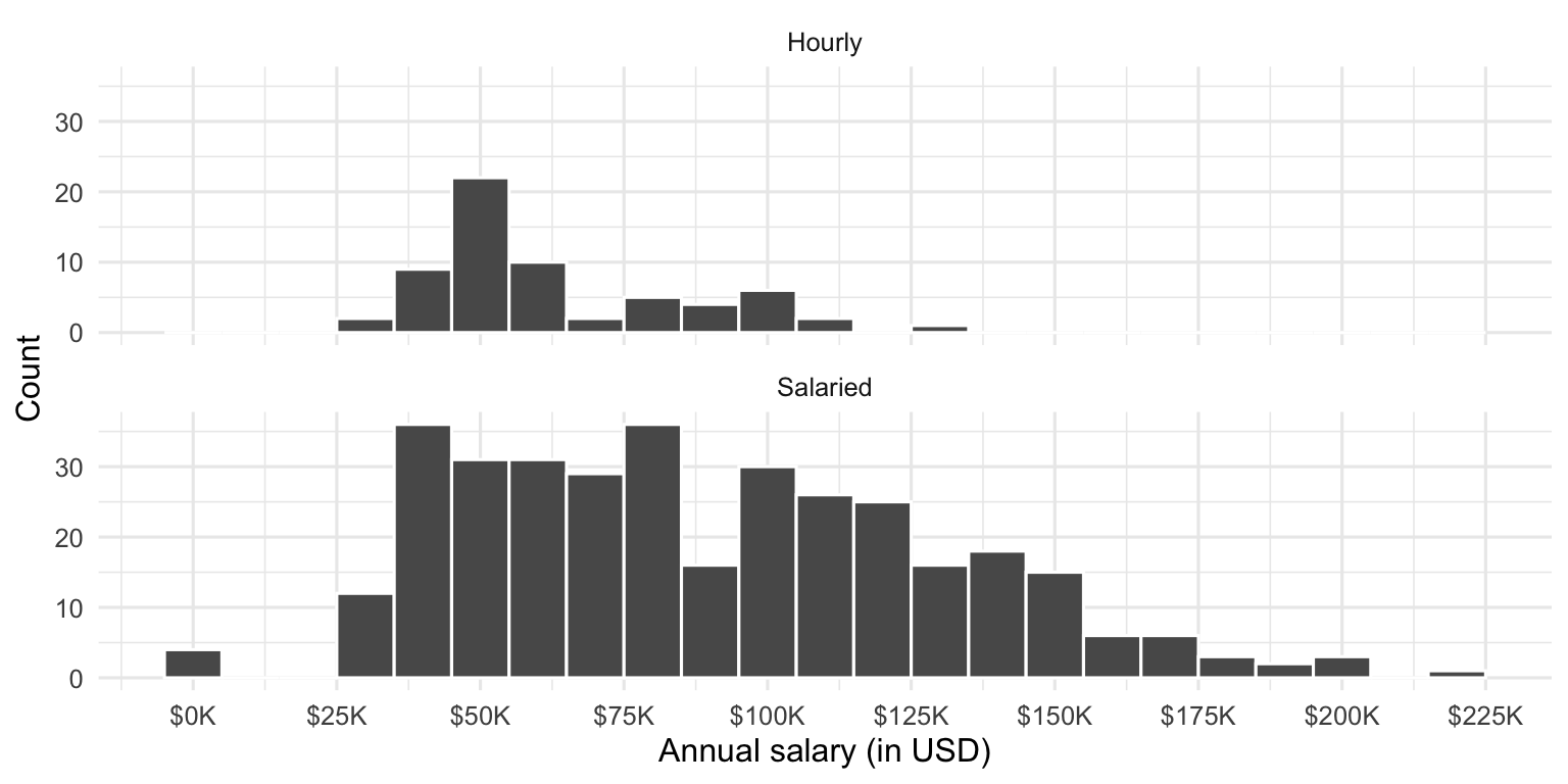
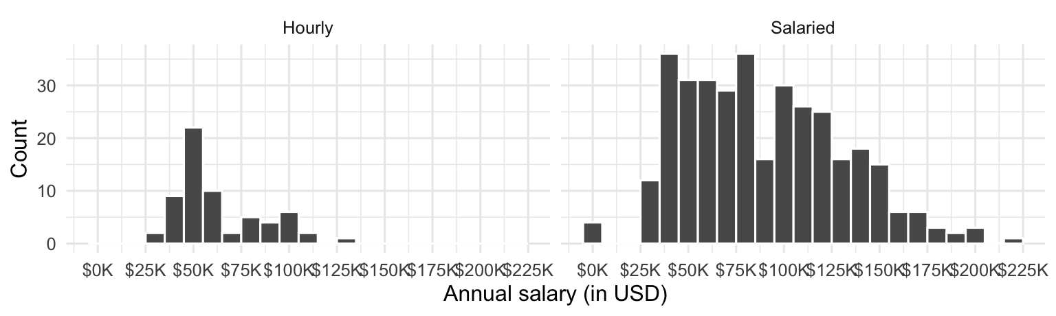
Figure 1 (a) and Figure 1 (b) show the distributions of annual salaries of hourly and salaried workers. The two figures show the same data, with the facets organized across rows and across columns. Which of the two figures is better for comparing the median annual salaries of hourly and salaried workers. Explain your reasoning.

Question 17

Suppose your teammate wrote the following code as part of their analysis of the data.

blizzard_salary |>
  group_by(salary_type) |>
  summarize(
    mean_annual_salary = mean(annual_salary),
    median_annual_salary = median(annual_salary)
  )

They then printed out the results shown below. Unfortunately one of the numbers got erased from the printout. It’s indicated with _____ below.

# A tibble: 2 × 3
  salary_type mean_annual_salary median_annual_salary
  <chr>                    <dbl>                <dbl>
1 Hourly                  63003.               54246.
2 Salaried                90183.               _____

Which of the following is the best estimate for that erased value?

30,000
50,000
80,000
100,000

Question 18

Which distribution of annual salaries has a higher standard deviation?

Hourly workers
Salaried workers
Roughly the same

Question 19

Which of the following alternate plots would also be useful for visualizing the distributions of annual salaries of hourly and salaried workers? Choose all that apply.

a. Box plots

b. Density plots

c. Pie charts

d. Waffle charts

e. Histograms

f. Scatterplots

Questions 20 - 22

Another teammate creates the following two plots.

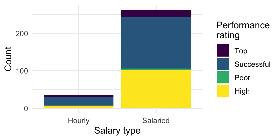
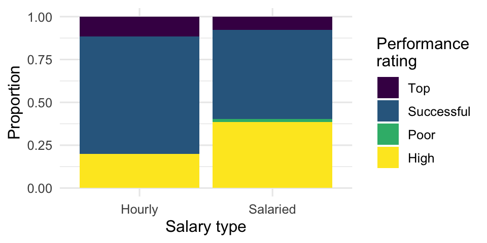
Question 20: Your teammate asks you for help deciding which one to use in the final report for visualizing the relationship between performance rating and salary type. In 1-3 sentences, can you help them make a decision, justify your choice, and write the narrative that should go with the plot?

Question 21: A friend with a keen eye points out that the number of observations in Figure 2 (a) seems lower than the total number of observations in blizzard_salary. What might be going on here? Explain your reasoning.

Question 22: Below are the proportions of performance ratings for hourly and salaried workers. Place these values in the corresponding segments in Figure 2 (b).

# A tibble: 4 × 3
  performance_rating Hourly Salaried
  <chr>               <dbl>    <dbl>
1 High                0.2     0.384 
2 Successful          0.686   0.521 
3 Top                 0.114   0.0760
4 Poor                0       0.0190

Question 23

You’re reviewing another team’s work and they made the following visualization:

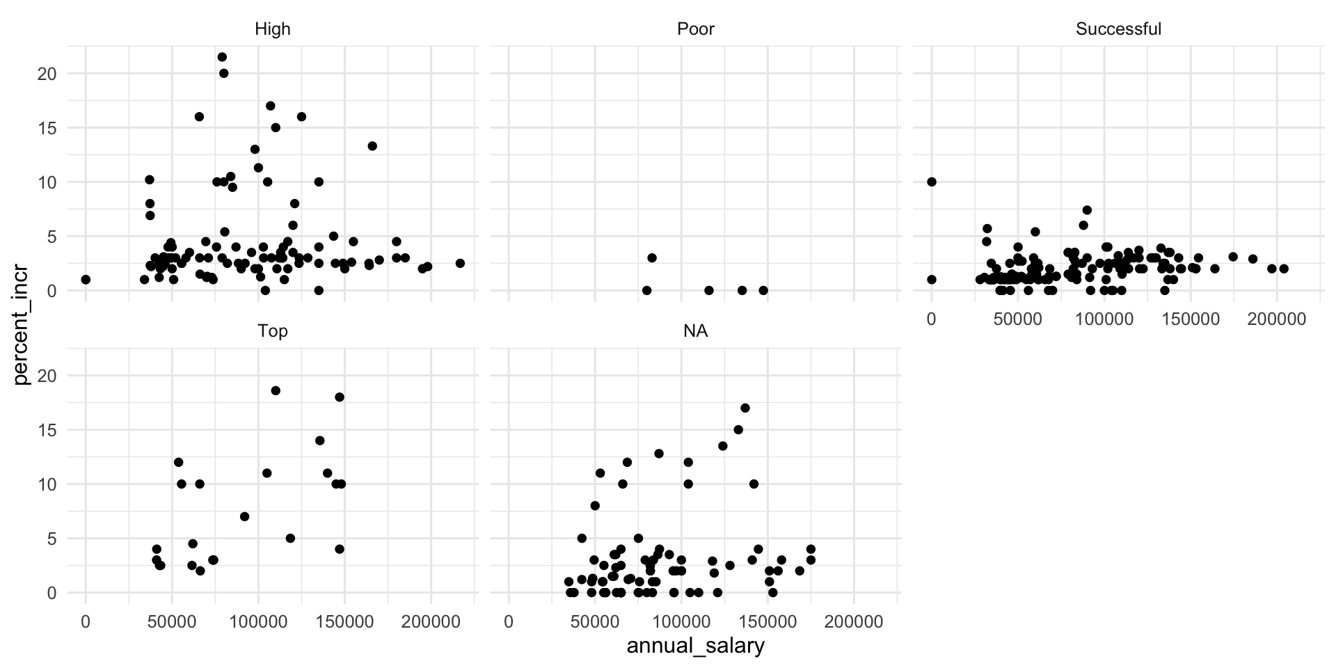
And they wrote the following interpretation for the relationship between annual salary and percent increase for Top performers:

The relationship is positive, having a higher salary results in a higher percent increase. There is one clear outlier.

Which of the following are the most accurate and helpful peer review notes for this interpretation? Choose all that apply.

The interpretation is complete and perfect, no changes needed!
The interpretation doesn’t mention the direction of the relationship.
The interpretation doesn’t mention the form of the relationship, which is linear.
The interpretation doesn’t mention the strength of the relationship, which is somewhat strong.
There isn’t a clear outlier in the plot. If any points stand out as potential outliers, more guidance should be given to the reader to identify them (e.g., salary and/or percent increase amount).
The interpretation is causal – we don’t know if the cause of the high percent increase is higher annual salary based on observational data. The causal direction might be the other way around, or there may be other factors contributing to the apparent relationship.

Question 24

You fit a model for predicting raises (percent_incr) from salaries (annual_salary). We’ll call this model raise_1_fit. A tidy output of the model is shown below.

# A tibble: 2 × 5
  term           estimate  std.error statistic   p.value
  <chr>             <dbl>      <dbl>     <dbl>     <dbl>
1 (Intercept)   1.87      0.432           4.33 0.0000194
2 annual_salary 0.0000155 0.00000452      3.43 0.000669

Which of the following is the best interpretation of the slope coefficient?

For every additional $1,000 of annual salary, the model predicts the raise to be higher, on average, by 1.55%.
For every additional $1,000 of annual salary, the raise goes up by 0.0155%.
For every additional $1,000 of annual salary, the model predicts the raise to be higher, on average, by 0.0155%.
For every additional $1,000 of annual salary, the model predicts the raise to be higher, on average, by 1.87%.

Question 25

You then fit a model for predicting raises (percent_incr) from salaries (annual_salary) and performance ratings (performance_rating). We’ll call this model raise_2_fit. Which of the following is definitely true based on the information you have so far?

Intercept of raise_2_fit is higher than intercept of raise_1_fit.
Slope of raise_2_fit is higher than RMSE of raise_1_fit.
Adjusted $R^2$ of raise_2_fit is higher than adjusted $R^2$ of raise_1_fit.
$R^2$ of raise_2_fit is higher $R^2$ of raise_1_fit.

Question 26

The tidy model output for the raise_2_fit model you fit is shown below.

# A tibble: 5 × 5
  term                            estimate  std.error statistic  p.value
  <chr>                              <dbl>      <dbl>     <dbl>    <dbl>
1 (Intercept)                   3.55       0.508           6.99 1.99e-11
2 annual_salary                 0.00000989 0.00000436      2.27 2.42e- 2
3 performance_ratingPoor       -4.06       1.42           -2.86 4.58e- 3
4 performance_ratingSuccessful -2.40       0.397          -6.05 4.68e- 9
5 performance_ratingTop         2.99       0.715           4.18 3.92e- 5

When your teammate sees this model output, they remark

“The coefficient for performance_ratingSuccessful is negative. That’s weird. I guess it means that people who get successful performance ratings get lower raises.”

How would you respond to your teammate?

Question 27

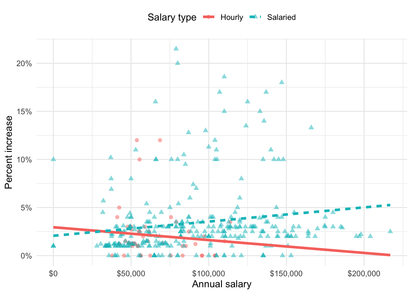
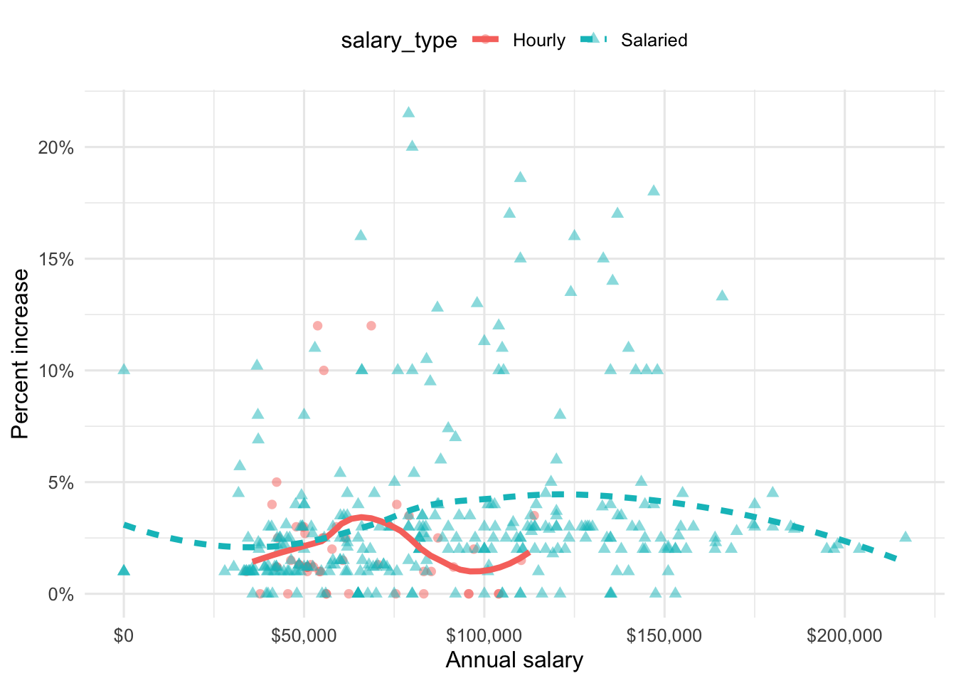
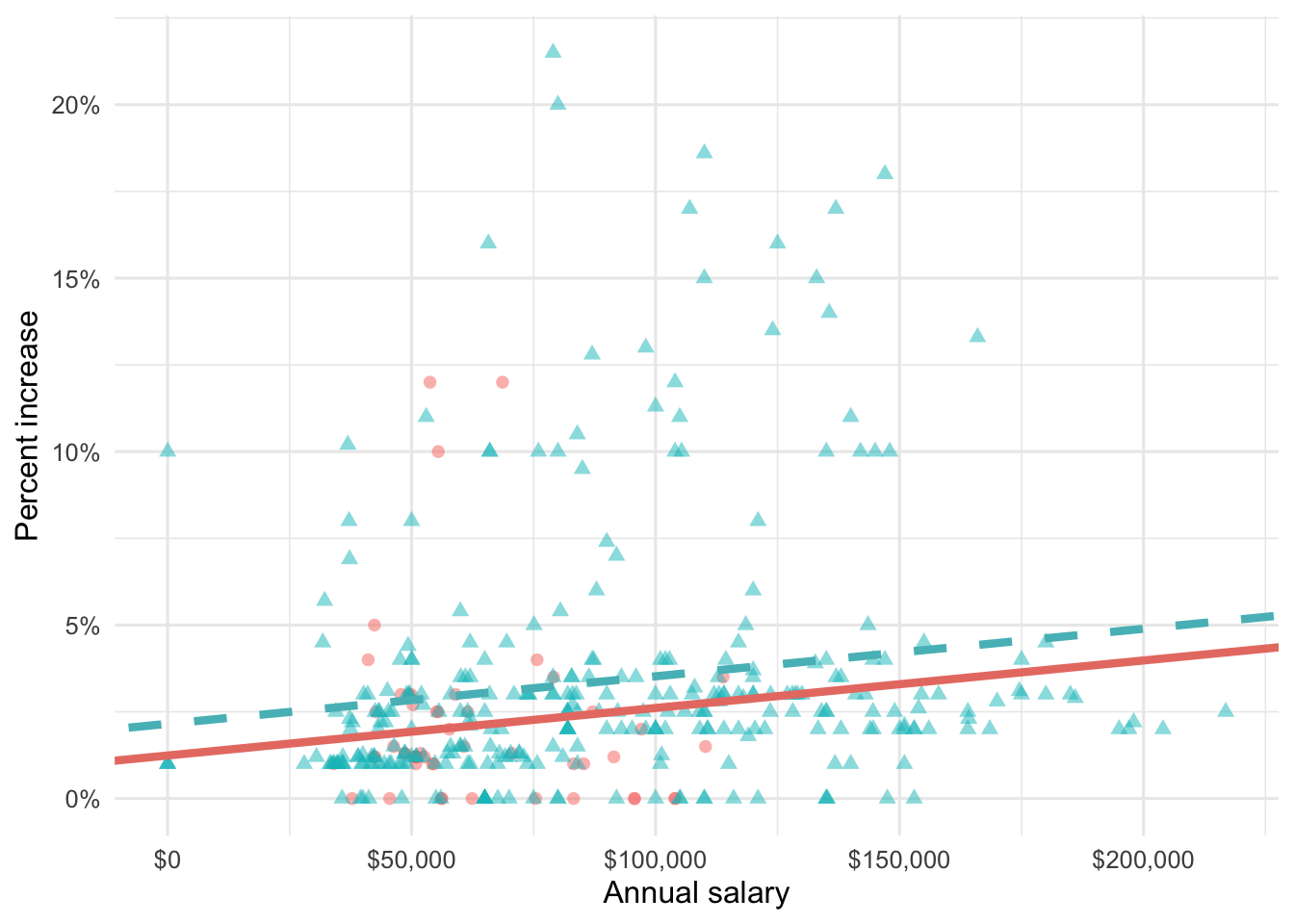
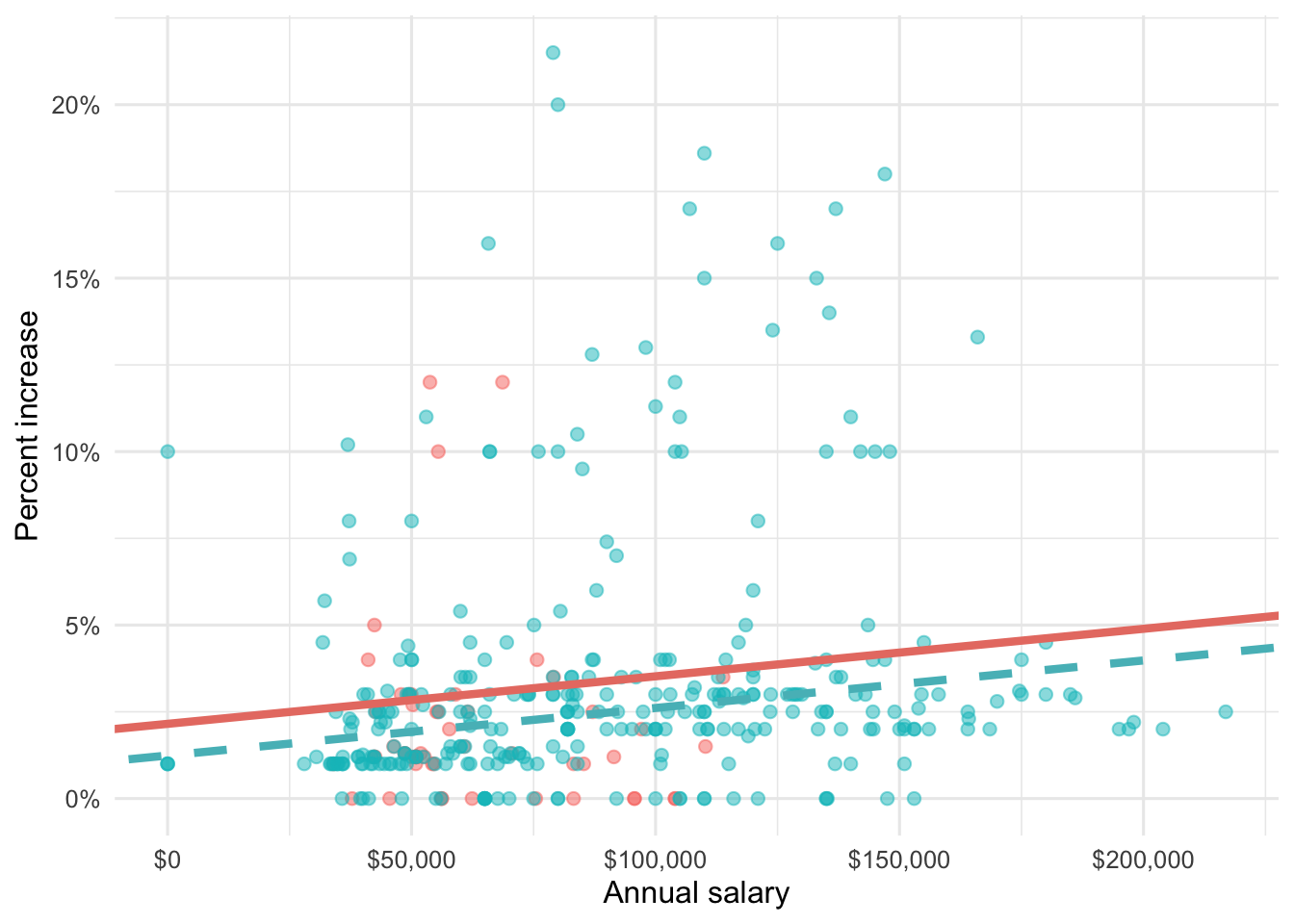
Suppose we fit a model to predict percent_incr from annual_salary and salary_type. A tidy output of the model is shown below.

# A tibble: 3 × 5
  term                 estimate  std.error statistic p.value
  <chr>                   <dbl>      <dbl>     <dbl>   <dbl>
1 (Intercept)         1.24      0.570           2.18 0.0300 
2 annual_salary       0.0000137 0.00000464      2.96 0.00329
3 salary_typeSalaried 0.913     0.544           1.68 0.0938

Which of the following visualizations represent this model? Explain your reasoning.

Question 28 (updated)

Suppose you now relevel the performance rating variable and fit a model to predict the natural log of percent increase, log(percent_incr), from performance rating. The model is called raise_4_fit.

You’re provided the following:

tidy(raise_4_fit) |>
  select(term, estimate) |>
  mutate(exp_estimate = exp(estimate))

# A tibble: 4 × 3
  term                         estimate exp_estimate
  <chr>                           <dbl>        <dbl>
1 (Intercept)                     -7.15     0.000786
2 performance_ratingSuccessful     6.93  1025.      
3 performance_ratingHigh           8.17  3534.      
4 performance_ratingTop            8.91  7438.

Based on this, which of the following is true?

a. The model predicts that the percentage increase employees with Successful performance get, on average, is higher by 10.25% compared to the employees with Poor performance rating.

b. The model predicts that the percentage increase employees with Successful performance get, on average, is higher by 6.93% compared to the employees with Poor performance rating.

c. The model predicts that the percentage increase employees with Successful performance get, on average, is higher by a factor of 1025 compared to the employees with Poor performance rating.

d. The model predicts that the percentage increase employees with Successful performance get, on average, is higher by a factor of 6.93 compared to the employees with Poor performance rating.

Movies

The data for this part comes from the Internet Movie Database (IMDB). Specifically, the data are a random sample of movies released between 1980 and 2020.

The name of the data frame used for this analysis is movies, and it contains the variables shown in Table 1.

Table 1: Data dictionary for movies

Variable	Description
`name`	name of the movie
`rating`	rating of the movie (R, PG, etc.)
`genre`	main genre of the movie.
`runtime`	duration of the movie
`year`	year of release
`release_date`	release date (YYYY-MM-DD)
`release_country`	release country
`score`	IMDB user rating
`votes`	number of user votes
`director`	the director
`writer`	writer of the movie
`star`	main actor/actress
`country`	country of origin
`budget`	the budget of a movie (some movies don’t have this, so it appears as 0)
`gross`	revenue of the movie
`company`	the production company

The first thirty rows of the movies data frame are shown in Table 2, with variable types suppressed (since we’ll ask about them later).

Table 2

First 30 rows of movies, with variable types suppressed.

# A tibble: 500 × 16
   name           score runtime genre     rating    release_country release_date
 1 Blue City        4.4 83 mins Action    R         United States   1986-05-02  
 2 Winter Sleep     8.1 196     Drama     Not Rated Turkey          2014-06-12  
 3 Rang De Basan…   8.1 167     Comedy    Not Rated United States   2006-01-26  
 4 Pokémon Detec…   6.6 104     Action    PG        United States   2019-05-10  
 5 A Bad Moms Ch…   5.6 104     Comedy    R         United States   2017-11-01  
 6 Replicas         5.5 107     Drama     PG-13     United States   2019-01-11  
 7 Windy City       5.8 103     Drama     R         Uruguay         1986-01-01  
 8 War for the P…   7.4 140     Action    PG-13     United States   2017-07-14  
 9 Tales from th…   6.4 98      Crime     R         United States   1995-05-24  
10 Fire with Fire   6.5 103     Drama     PG-13     United States   1986-05-09  
11 Raising Helen    6   119     Comedy    PG-13     United States   2004-05-28  
12 Feeling Minne…   5.4 99      Comedy    R         United States   1996-09-13  
13 The Babe         5.9 115     Biography PG        United States   1992-04-17  
14 The Real Blon…   6   105     Comedy    R         United States   1998-02-27  
15 To vlemma tou…   7.6 176     Drama     Not Rated United States   1997-11-01  
16 Going the Dis…   6.3 102     Comedy    R         United States   2010-09-03  
17 Jung on zo       6.8 103     Action    R         Hong Kong       1993-06-24  
18 Rita, Sue and…   6.5 93      Comedy    R         United Kingdom  1987-05-29  
19 Phone Booth      7   81      Crime     R         United States   2003-04-04  
20 Happy Death D…   6.6 96      Comedy    PG-13     United States   2017-10-13  
21 Barely Legal     4.7 90      Comedy    R         Thailand        2006-05-25  
22 Three Kings      7.1 114     Action    R         United States   1999-10-01  
23 Menace II Soc…   7.5 97      Crime     R         United States   1993-05-26  
24 Four Rooms       6.8 98      Comedy    R         United States   1995-12-25  
25 Quartet          6.8 98      Comedy    PG-13     United States   2013-03-01  
26 Tape             7.2 86      Drama     R         Denmark         2002-07-12  
27 Marked for De…   6   93      Action    R         United States   1990-10-05  
28 Congo            5.2 109     Action    PG-13     United States   1995-06-09  
29 Stop-Loss        6.4 112     Drama     R         United States   2008-03-28  
30 Con Air          6.9 115     Action    R         United States   1997-06-06  
# ℹ 470 more rows
# ℹ 9 more variables: budget, gross, votes, year,
#   director, writer, star, company, country

Score vs. runtime

In this part, we fit a model predicting score from runtime and name it score_runtime_fit.

score_runtime_fit <- linear_reg() |>
  fit(score ~ runtime, data = movies)

Figure 4 visualizes the relationship between score and runtime as well as the linear model for predicting score from runtime. The first three movies in Table 2 are labeled in the visualization as well. Answer all questions in this part based on Figure 4.

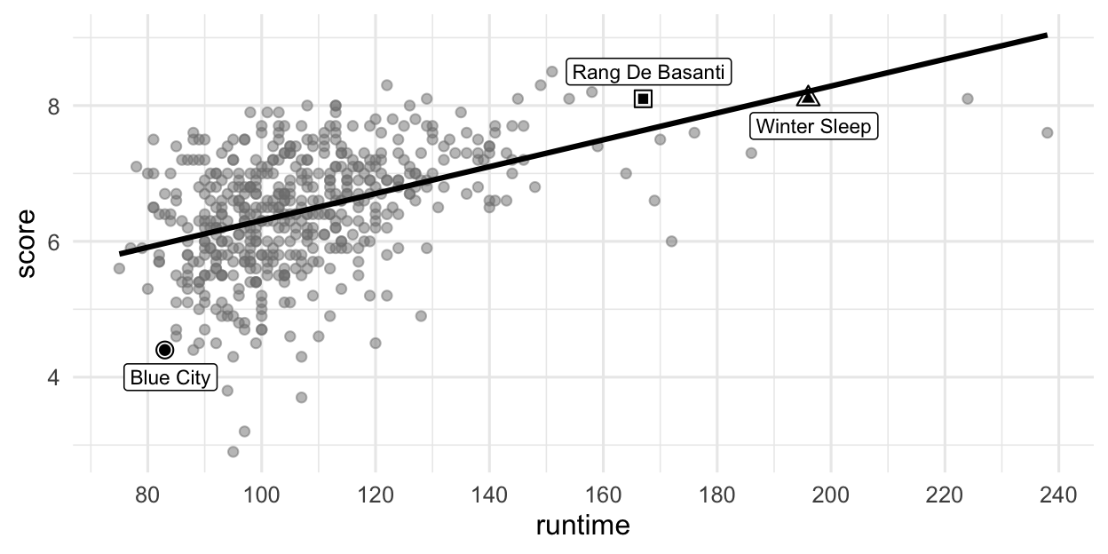
Figure 4: Scatterplot of `score` vs. `runtime` for `movies`.

Question 29

Based on this model, order the three labeled movies in Figure 4 in decreasing order of the magnitude (absolute value) of their residuals.

Winter Sleep > Rang De Basanti > Blue City
Winter Sleep > Blue City > Rang De Basanti
Rang De Basanti > Winter Sleep > Blue City
Blue City > Winter Sleep > Rang De Basanti
Blue City > Rang De Basanti > Winter Sleep

Question 30

The R-squared for the model visualized in Figure 4 is 31%. Which of the following is the best interpretation of this value?

31% of the variability in movie runtimes is explained by their scores.
31% of the variability in movie scores is explained by their runtime.
The model accurately predicts scores of 31% of the movies in this sample.
The model accurately predicts scores of 31% of all movies.
The correlation between scores and runtimes of movies is 0.31.

Score vs. runtime or year

The visualizations below show the relationship between score and runtime as well as score and year, respectively. Additionally, the lines of best fit are overlaid on the visualizations.

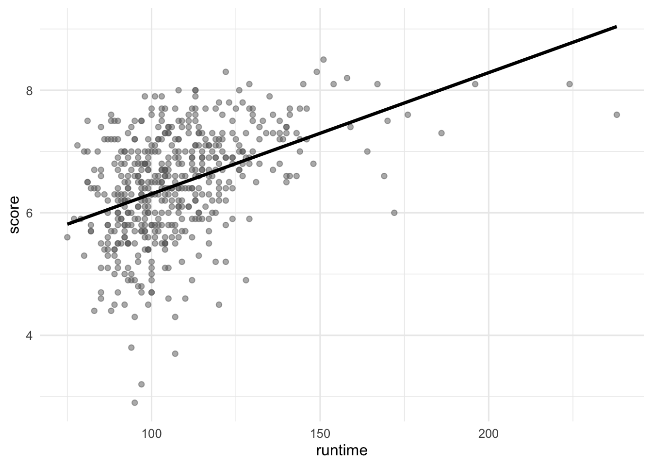
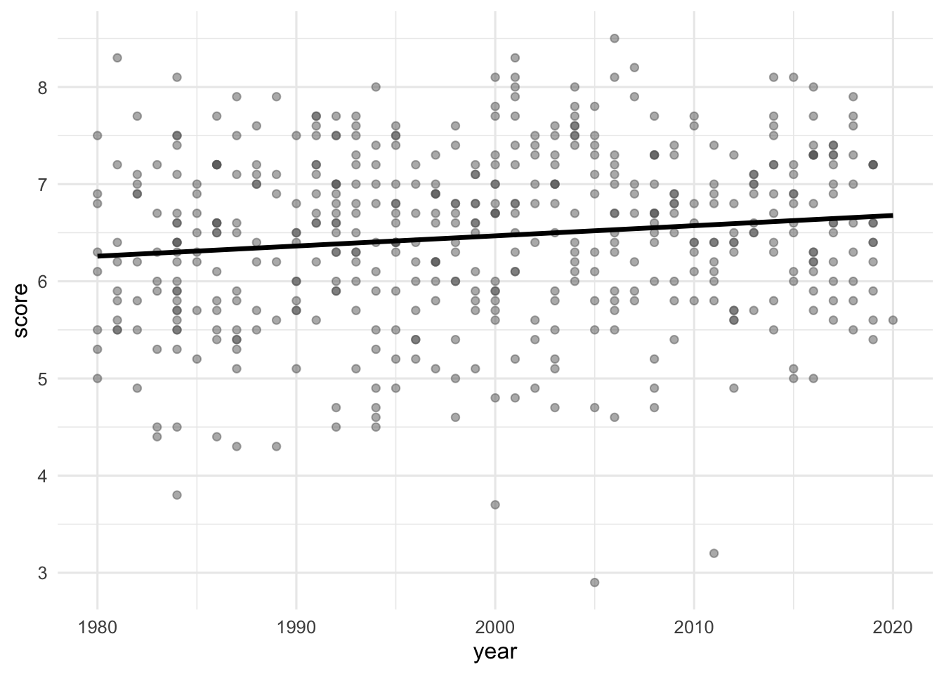
The correlation coefficients of these relationships are calculated below, though some of the code and the output are missing. Answer all questions in this part based on the code and output shown below.

movies |>
  summarize(
    r_score_runtime = cor(runtime, score),
    r_score_year = cor(year, score)
  )

# A tibble: 1 × 2
  r_score_runtime r_score_year
            <dbl>        <dbl>
1           0.434. __blank_2__

Question 31

What can we say about the value that goes in __blank_2__?

NA
A value between 0 and 0.434.
A value between 0.434 and 1.
A value between 0 and -0.434.
A value between -1 and -0.434.

Score vs. runtime and rating

In this part, we fit a model predicting score from runtime and rating (categorized as G, PG, PG-13, R, NC-17, and Not Rated), and name it score_runtime_rating_fit.

The model output for score_runtime_rating_fit is shown in Table 3. Answer all questions in this part based on Table 3.

Table 3: Regression output for score_runtime_rating_fit.

term	estimate	std.error	statistic	p.value
(Intercept)	4.525	0.332	13.647	0.000
runtime	0.021	0.002	10.702	0.000
ratingPG	-0.189	0.295	-0.642	0.521
ratingPG-13	-0.452	0.292	-1.547	0.123
ratingR	-0.257	0.285	-0.901	0.368
ratingNC-17	-0.355	0.486	-0.730	0.466
ratingNot Rated	-0.282	0.328	-0.860	0.390

Question 32

Which of the following is TRUE about the intercept of score_runtime_rating_fit? Select all that are true.

Keeping runtime constant, G-rated movies are predicted to score, on average, 4.525 points.
Keeping runtime constant, movies without a rating are predicted to score, on average, 4.525 points.
Movies without a rating that are 0 minutes in length are predicted to score, on average, 4.525 points.
All else held constant, movies that are 0 minutes in length are predicted to score, on average, 4.525 points.
G-rated movies that are 0 minutes in length are predicted to score, on average, 4.525 points.

Question 33

Which of the following is the best interpretation of the slope of runtime in score_runtime_rating_fit?

All else held constant, as runtime increases by 1 minute, the score of the movie increases by 0.021 points.
For G-rated movies, all else held constant, as runtime increases by 1 minute, we predict the score of the movie to be higher by 0.021 points on average.
All else held constant, for each additional minute of runtime, movie scores will be higher by 0.021 points on average.
G-rated movies that are 0 minutes in length are predicted to score 0.021 points on average.
For each higher level of rating, the movie scores go up by 0.021 points on average.

Question 34

Fill in the blank:

R-squared for score_runtime_rating_fit (the model predicting score from runtime and rating) _________ the R-squared the model score_runtime_fit (for predicting score from runtime alone).

is less than
is equal to
is greater than
cannot be compared (based on the information provided) to
is both greater than and less than

Question 35

The model score_runtime_rating_fit (the model predicting score from runtime and rating) can be visualized as parallel lines for each level of rating. Which of the following is the equation of the line for R-rated movies?

$\widehat{score} = (4.525 - 0.257) + 0.021 \times runtime$
$score = (4.525 - 0.257) + 0.021 \times runtime$
$\widehat{score} = 4.525 + (0.021 - 0.257) \times runtime$
$score = 4.525 + (0.021 - 0.257) \times runtime$
$\widehat{score} = (4.525 + 0.021) - 0.257 \times runtime$

Selection

Let say we want to predict score and we are considering using runtime, budget, and year to do it. So we compute the adjusted $R^2$ for every possible additive model, and we get

Model	Adjusted $R^2$
`score ~ 1`	0
`score ~ runtime`	0.1867485
`score ~ budget`	0.0010866
`score ~ year`	0.0156397
`score ~ runtime + budget`	0.1719674
`score ~ runtime + year`	0.1899246
`score ~ budget + year`	0.0043752
`score ~ runtime + budget + year`	0.1745898

Question 36

Which model is “best”?

Question 37

Which model will you select if you follow forward stepwise selection?

Question 38

Which model will you select if you follow backward elimination?

Footnotes

“Doink doink” is the scene and episode introductory sound on the Law & Order series. If you’ve never heard it, you’re not at any disadvantage for the exam. If you’ve ever heard it, good luck getting it out of your head!↩︎