Observational studies

Lecture 13

Author

Affiliation

Josh Lim and John Zito

Duke University
STA 101 Fall 2026

Recap

Last lecture: RCTs

• We showed that randomization is incredibly powerful: it makes \(Z \perp X\), so any difference in \(Y\) between groups must be due to treatment.

• This gave us the license to say things like: “receiving VWG OIT causes an increase in max tolerated wheat protein dose;”

• Today: what happens when we can’t randomize?

When randomization isn’t possible

• Ethical: you cannot randomly assign people to smoke, to not receive healthcare, or to experience childhood poverty;

• Practical: policy changes happen at scale. You can’t “randomize” a country’s tax policy;

• Historical: many causal questions are about events that already happened;

• Most real-world causal questions are answered with observational data.

Observational Studies

What is an observational study?

• In an observational study, treatment is not assigned by the researcher. Subjects choose, or are assigned by nature or circumstance;

• Examples: surveys (including the Census), electronic health records, administrative data;

• Almost any dataset you encounter “in the wild” can be framed as an observational study. You just have to define what the treatment is;

• Key advantage over RCTs: easier and cheaper to collect, often with much larger sample sizes.

The core issue

Without randomization, \(Z\) is not independent of \(X\). People who receive treatment differ systematically from those who don’t.

. . .

Person	\(Z\) (Duke?)	\(X\) (Read Percy Jackson?)	\(Y\) (Odyssey rating)
A	1	Yes	9
B	1	Yes	8
C	0	No	5
D	0	No	6

. . .

Is the difference in Odyssey ratings because of Duke vs. UNC or because of Percy Jackson?

A concrete example

• \(Z\): attended Duke (vs. UNC); \(Y\): rating of the new Odyssey movie; \(X\): read Percy Jackson as a kid;

• Duke students happen to be much more likely to have read Percy Jackson. \(Z\) and \(X\) are perfectly aligned;

• Percy Jackson fans also tend to rate the Odyssey higher. \(X\) affects \(Y\);

• So the naive comparison (“Duke students rate the Odyssey higher”) actually reflects Percy Jackson fandom, not school identity;

• This is confounding: \(X \to Z\) and \(X \to Y\), creating a spurious association between \(Z\) and \(Y\).

Key takeaway

• In an observational study, a naive difference in group means is not a valid causal estimate;

• We need to adjust for confounders \(X\) to recover the true treatment effect;

• The rest of today: two strategies for doing that.

Matching

The idea of matching

Recall from last lecture: randomization balanced the covariates. The only systematic difference between groups was the treatment.

. . .

Our goal in observational studies: emulate that balance without running an experiment.

. . .

How? Matching.

Matching

• For each treated unit, find one or more control units that look similar on \(X\);

• This creates two new comparable cohorts: a matched treated group and a matched control group;

• Analyze the outcome across these cohorts, just as you would in a randomized experiment;

• Key requirement: matching only works if we have measured all important confounders. This is a strong, untestable assumption.

Let’s hold on this for a second

• One of the advantages of a randomized experiment is that it can produce a plausible causal estimate regardless whether or not you measured all confounders;
• Now, in order to produce a plausible causal estimate for observational data, you must assume that all confounders were measured. Otherwise it doesn’t work;
• So really, causal inference depends more on study design and data collection than on the particular statistical technique you use;
• And it’s hard!

New package!

MatchIt provides a simple and straightforward interface to various methods of matching for covariate balance in observational studies.

The LaLonde Study

Context

LaLonde (1986) evaluated the National Supported Work (NSW) program, a 1970s job training intervention for disadvantaged workers.

• Cohort: Disadvantaged workers (long-term unemployed, ex-offenders, welfare recipients);

• Design: The original NSW had a randomized arm, but LaLonde compared its estimates against observational comparison groups drawn from national surveys, showing how badly naive methods can fail;

• Treatment (\(Z = 1\)): Participation in the NSW job training program;

• Control (\(Z = 0\)): Non-participants drawn from observational comparison groups;

• Outcome (\(Y\)): Earnings in 1978 (re78);

• Covariates (\(X\)): Age, education, race, marital status, prior earnings (re74, re75).

Data

data("lalonde", package = "MatchIt")
glimpse(lalonde)

Rows: 614
Columns: 9
$ treat    <int> 1, 1, 1, 1, 1, 1, 1, 1, 1, 1, 1, 1, 1, 1, 1, 1, 1, 1, 1, 1, 1…
$ age      <int> 37, 22, 30, 27, 33, 22, 23, 32, 22, 33, 19, 21, 18, 27, 17, 1…
$ educ     <int> 11, 9, 12, 11, 8, 9, 12, 11, 16, 12, 9, 13, 8, 10, 7, 10, 13,…
$ race     <fct> black, hispan, black, black, black, black, black, black, blac…
$ married  <int> 1, 0, 0, 0, 0, 0, 0, 0, 0, 1, 0, 0, 0, 1, 0, 0, 0, 0, 0, 0, 0…
$ nodegree <int> 1, 1, 0, 1, 1, 1, 0, 1, 0, 0, 1, 0, 1, 1, 1, 1, 0, 1, 0, 0, 1…
$ re74     <dbl> 0, 0, 0, 0, 0, 0, 0, 0, 0, 0, 0, 0, 0, 0, 0, 0, 0, 0, 0, 0, 0…
$ re75     <dbl> 0, 0, 0, 0, 0, 0, 0, 0, 0, 0, 0, 0, 0, 0, 0, 0, 0, 0, 0, 0, 0…
$ re78     <dbl> 9930.0460, 3595.8940, 24909.4500, 7506.1460, 289.7899, 4056.4…

• treat: 1 = job training, 0 = no training
• re78: earnings in 1978 (outcome \(Y\))
• age, educ, re74, re75, …: pre-treatment covariates (\(X\))

Naive estimate

lalonde |>
  group_by(treat) |>
  summarise(mean_earnings = mean(re78))

# A tibble: 2 × 2
  treat mean_earnings
  <int>         <dbl>
1     0         6984.
2     1         6349.

• The naive difference suggests training DECREASES earnings! (huh?)

• But are the two groups actually comparable before treatment?

Your turn

Look at the balance table below. Which variables show the largest differences between treated and control groups? What does this tell us about the naive estimate?

lalonde |>
  group_by(treat) |>
  summarise(
    mean_age  = mean(age),
    mean_educ = mean(educ),
    mean_re74 = mean(re74),
    mean_re75 = mean(re75)
  )

# A tibble: 2 × 5
  treat mean_age mean_educ mean_re74 mean_re75
  <int>    <dbl>     <dbl>     <dbl>     <dbl>
1     0     28.0      10.2     5619.     2466.
2     1     25.8      10.3     2096.     1532.

What the imbalance tells us

• Treated individuals have substantially lower prior earnings (re74, re75) than controls;

• The control group (from national surveys) is richer and more educated on average;

• A naive comparison overstates the earnings gap. The treated group is catching up from a lower baseline, not just benefiting from training;

• We need to adjust for these differences before drawing causal conclusions.

Nearest-neighbor matching

m_out <- matchit(
  treat ~ age + educ + re74 + re75,
  data   = lalonde,
  method = "nearest",
  distance = "mahalanobis"
)
summary(m_out, un = FALSE)

Call:
matchit(formula = treat ~ age + educ + re74 + re75, data = lalonde, 
    method = "nearest", distance = "mahalanobis")

Summary of Balance for Matched Data:
     Means Treated Means Control Std. Mean Diff. Var. Ratio eCDF Mean eCDF Max
age        25.8162       25.4054          0.0574     0.7447    0.0351   0.1351
educ       10.3459       10.5027         -0.0780     0.8938    0.0134   0.1081
re74     2095.5737     2545.1934         -0.0920     1.2585    0.0746   0.3405
re75     1532.0553     1651.6935         -0.0372     1.3200    0.0408   0.1838
     Std. Pair Dist.
age           0.3143
educ          0.2285
re74          0.2024
re75          0.1648

Sample Sizes:
          Control Treated
All           429     185
Matched       185     185
Unmatched     244       0
Discarded       0       0

Estimate on matched data

m_data <- match.data(m_out)

linear_reg() |>
  fit(re78 ~ treat, data = m_data) |>
  tidy()

# A tibble: 2 × 5
  term        estimate std.error statistic  p.value
  <chr>          <dbl>     <dbl>     <dbl>    <dbl>
1 (Intercept)    5842.      529.    11.0   1.09e-24
2 treat           507.      748.     0.678 4.98e- 1

• After matching, treated and control units are much more comparable on \(X\);

• This estimate is our best causal guess under the no-unmeasured-confounders assumption;

• Compare to the naive estimate. Confounding matters!

Propensity scores

The curse of dimensionality

• Covariate matching works well when \(X\) has only a few variables;

• With many covariates, it becomes nearly impossible to find good matches. Imagine trying to match on 10 variables simultaneously!

• Example: match exactly on age, education, prior earnings, race, marital status, region, …

• The probability of finding a near-identical control unit vanishes as the number of covariates grows;

• We need a smarter approach.

The propensity score

• Instead of matching on the full \(X\) vector, collapse it to a single number;

• The propensity score:

  \[e(X) = P(Z = 1 \mid X);\]

• The probability of receiving treatment, given covariates;

• Matching on this one number is sufficient to achieve balance on all of \(X\);

• In a randomized experiment, \(e(X) = 0.5\) for everyone. Randomization makes treatment equally likely regardless of \(X\).

But how do we estimate it?

• Every unit has a true \(e(X) = P(Z = 1 \mid X)\). We don’t observe it directly;

• Goal: estimate \(\hat{e}(X)\), the predicted probability of treatment given covariates;

• We want to model \(P(Z = 1)\) from \(X\) … what does that sound like?

• Logistic regression! We already know how to do this.

Estimating the propensity score

We estimate \(e(X)=P(Z=1\mid X)\) via logistic regression:

\[\log\frac{\hat{e}(X)}{1 - \hat{e}(X)} = {b_0} + {b_1} X_1 + \cdots + {b_p} X_p;\]

• Fit logistic regression of \(Z\) on \(X\);

• Predicted probabilities \(\hat{e}(X_i)\) are the estimated propensity scores;

• Match treated and control units with similar \(\hat{e}(X)\).

The workflow

1. Fit a logistic regression model: \(Z \sim X_1 + \cdots + X_p\);
2. Extract predicted probabilities as propensity scores;
3. Match treated to control units with similar scores;
4. Check balance on \(X\) in the matched sample;
5. Estimate the treatment effect on the matched data.

Step 1 & 2: fit model, get scores

ps_fit <- logistic_reg() |>
  fit(factor(treat) ~ age + educ + re74 + re75, data = lalonde)

lalonde <- lalonde |>
  mutate(ps = predict(ps_fit, type = "prob", new_data = lalonde)$.pred_1)

lalonde |>
  group_by(treat) |>
  summarise(mean_ps = mean(ps), sd_ps = sd(ps))

# A tibble: 2 × 3
  treat mean_ps  sd_ps
  <int>   <dbl>  <dbl>
1     0   0.279 0.126 
2     1   0.354 0.0901

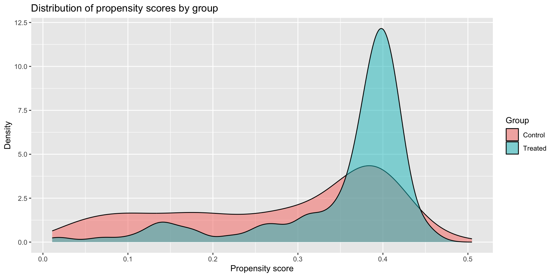
Visualize the scores

ggplot(
  lalonde,
  aes(x = ps, fill = factor(treat, labels = c("Control", "Treated")))
) +
  geom_density(alpha = 0.5) +
  labs(
    x     = "Propensity score",
    y     = "Density",
    fill  = "Group",
    title = "Distribution of propensity scores by group"
  )

Step 3 & 4: match and check balance

ps_match <- matchit(
  treat ~ age + educ + re74 + re75,
  data     = lalonde,
  method   = "nearest",
  distance = "glm"
)

summary(ps_match, un = FALSE)

Call:
matchit(formula = treat ~ age + educ + re74 + re75, data = lalonde, 
    method = "nearest", distance = "glm")

Summary of Balance for Matched Data:
         Means Treated Means Control Std. Mean Diff. Var. Ratio eCDF Mean
distance        0.3536        0.3523          0.0141     1.0160    0.0088
age            25.8162       25.2811          0.0748     0.4690    0.0801
educ           10.3459       10.4486         -0.0511     0.6392    0.0208
re74         2095.5737     2137.7507         -0.0086     1.2576    0.0365
re75         1532.0553     1385.2355          0.0456     1.7520    0.0379
         eCDF Max Std. Pair Dist.
distance   0.0757          0.0179
age        0.2486          1.4014
educ       0.0973          1.0673
re74       0.2541          0.1778
re75       0.1946          0.6412

Sample Sizes:
          Control Treated
All           429     185
Matched       185     185
Unmatched     244       0
Discarded       0       0

Step 5: estimate the treatment effect

ps_data <- match.data(ps_match)

linear_reg() |>
  fit(re78 ~ treat, data = ps_data) |>
  tidy()

# A tibble: 2 × 5
  term        estimate std.error statistic  p.value
  <chr>          <dbl>     <dbl>     <dbl>    <dbl>
1 (Intercept)    5988.      533.    11.2   2.38e-25
2 treat           362.      754.     0.479 6.32e- 1

• After propensity score matching, we have a valid causal estimate (under no unmeasured confounders);

• This scales to many covariates, unlike direct covariate matching;

• Always check balance after matching. If balance is poor, improve the propensity score model.

Limitations of observational studies

• No unmeasured confounders: the key assumption is untestable. If an important confounder is missing from \(X\), our estimate is still biased;

• Bad controls: only include pre-treatment variables in \(X\). Never include variables caused by \(Z\);

• Model dependence: the propensity score model matters. Wrong specification leads to poor balance and biased estimates;

• RCTs are still the gold standard; observational methods are our best option when experiments are impossible.

Key takeaways

• Observational studies require careful adjustment for confounders \(X\);

• Covariate matching: find control units similar on \(X\) directly. Works well with few covariates;

• Propensity score matching: match on \(P(Z = 1 \mid X)\). Scales to high dimensions;

• Both require no unmeasured confounders, an assumption that must be argued for, not tested from data;

• Now you have two tools to draw causal conclusions!