Exploratory Data Analysis, Part II
Lecture 3
Today’s example
So far…
| Data set | Occasion | Source | A row was a… |
|---|---|---|---|
age_guesses |
Lecture 0 | file | 101 student |
card_krueger |
Lecture 1 | file | restaurant |
pokemon |
Lab 0 | file | Pokémon |
penguins |
Lab 0 | package | penguin |
nc_county |
Lab1, HW 1 | file | NC county |
bechdel |
Lecture 2+ | file | film |
gerrymander |
Today | package | US congressional district |
Packages
- For the data: usdata
Data: gerrymander
gerrymander# A tibble: 435 × 12
district last_name first_name party16 clinton16 trump16 dem16 state party18
<chr> <chr> <chr> <chr> <dbl> <dbl> <dbl> <chr> <chr>
1 AK-AL Young Don R 37.6 52.8 0 AK R
2 AL-01 Byrne Bradley R 34.1 63.5 0 AL R
3 AL-02 Roby Martha R 33 64.9 0 AL R
4 AL-03 Rogers Mike D. R 32.3 65.3 0 AL R
5 AL-04 Aderholt Rob R 17.4 80.4 0 AL R
6 AL-05 Brooks Mo R 31.3 64.7 0 AL R
7 AL-06 Palmer Gary R 26.1 70.8 0 AL R
8 AL-07 Sewell Terri D 69.8 28.6 1 AL D
9 AR-01 Crawford Rick R 30.2 65 0 AR R
10 AR-02 Hill French R 41.7 52.4 0 AR R
# ℹ 425 more rows
# ℹ 3 more variables: dem18 <dbl>, flip18 <dbl>, gerry <fct>What is gerrymandering?
JZ’s tour of the USA
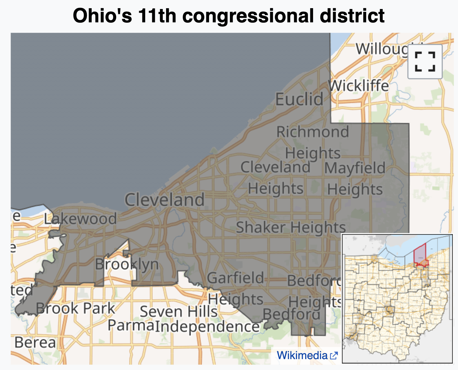
JZ’s tour of the USA
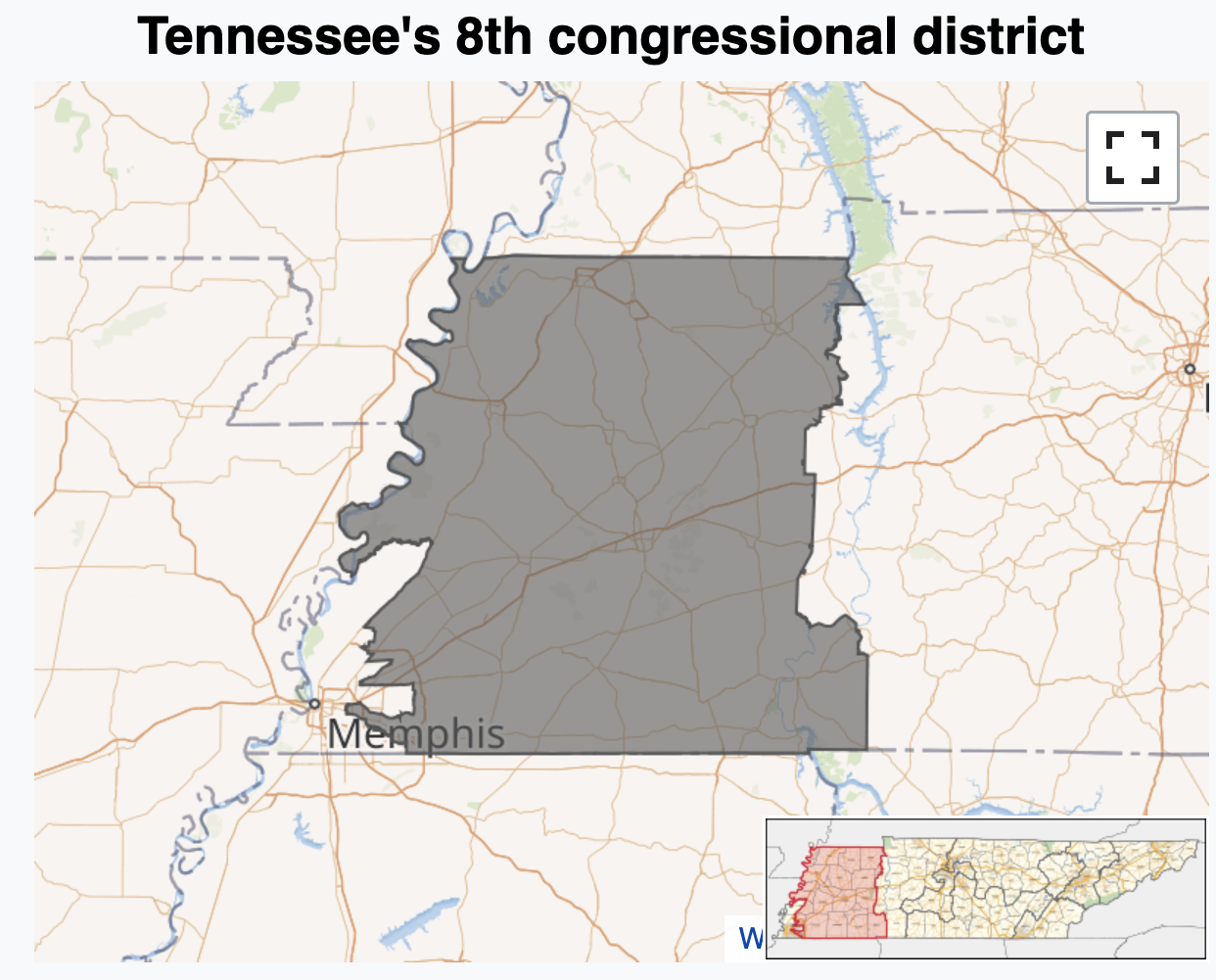
JZ’s tour of the USA
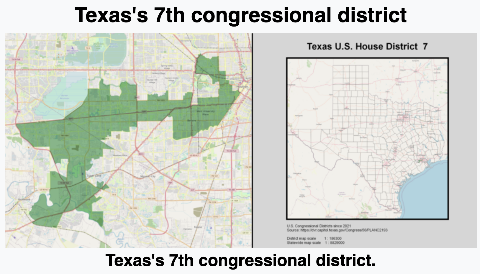
JZ’s tour of the USA
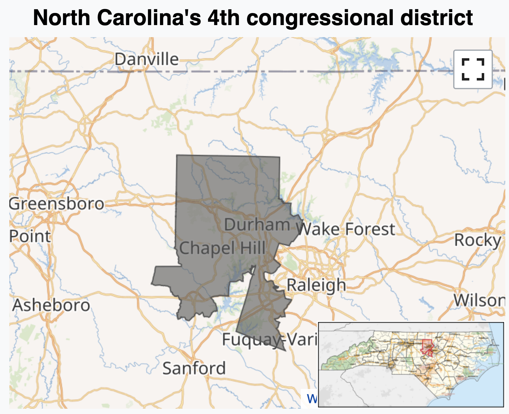
Data: gerrymander
What is a good first function to use to get to know a dataset?
glimpse(gerrymander)Rows: 435
Columns: 12
$ district <chr> "AK-AL", "AL-01", "AL-02", "AL-03", "AL-04", "AL-05", "AL-0…
$ last_name <chr> "Young", "Byrne", "Roby", "Rogers", "Aderholt", "Brooks", "…
$ first_name <chr> "Don", "Bradley", "Martha", "Mike D.", "Rob", "Mo", "Gary",…
$ party16 <chr> "R", "R", "R", "R", "R", "R", "R", "D", "R", "R", "R", "R",…
$ clinton16 <dbl> 37.6, 34.1, 33.0, 32.3, 17.4, 31.3, 26.1, 69.8, 30.2, 41.7,…
$ trump16 <dbl> 52.8, 63.5, 64.9, 65.3, 80.4, 64.7, 70.8, 28.6, 65.0, 52.4,…
$ dem16 <dbl> 0, 0, 0, 0, 0, 0, 0, 1, 0, 0, 0, 0, 1, 0, 1, 0, 0, 0, 1, 0,…
$ state <chr> "AK", "AL", "AL", "AL", "AL", "AL", "AL", "AL", "AR", "AR",…
$ party18 <chr> "R", "R", "R", "R", "R", "R", "R", "D", "R", "R", "R", "R",…
$ dem18 <dbl> 0, 0, 0, 0, 0, 0, 0, 1, 0, 0, 0, 0, 1, 1, 1, 0, 0, 0, 1, 0,…
$ flip18 <dbl> 0, 0, 0, 0, 0, 0, 0, 0, 0, 0, 0, 0, 0, 1, 0, 0, 0, 0, 0, 0,…
$ gerry <fct> mid, high, high, high, high, high, high, high, mid, mid, mi…Data: gerrymander
Rows: Congressional districts
-
Columns:
Congressional district and state
2016 election: winning party, % for Clinton, % for Trump, whether a Democrat won the House election, name of election winner
2018 election: winning party, whether a Democrat won the 2018 House election
Whether a Democrat flipped the seat in the 2018 election
Prevalence of gerrymandering: low, mid, and high
Variable types: district
| Variable | Type |
|---|---|
district |
categorical, ID |
last_name |
|
first_name |
|
party16 |
|
clinton16 |
|
trump16 |
|
dem16 |
|
state |
|
party18 |
|
dem18 |
|
flip18 |
|
gerry |
Congressional district:
gerrymander |>
select(district)# A tibble: 435 × 1
district
<chr>
1 AK-AL
2 AL-01
3 AL-02
4 AL-03
5 AL-04
6 AL-05
7 AL-06
8 AL-07
9 AR-01
10 AR-02
# ℹ 425 more rowsVariable types: last_name
| Variable | Type |
|---|---|
district |
categorical, ID |
last_name |
categorical, ID |
first_name |
|
party16 |
|
clinton16 |
|
trump16 |
|
dem16 |
|
state |
|
party18 |
|
dem18 |
|
flip18 |
|
gerry |
Last name of 2016 election winner:
gerrymander |>
select(last_name)# A tibble: 435 × 1
last_name
<chr>
1 Young
2 Byrne
3 Roby
4 Rogers
5 Aderholt
6 Brooks
7 Palmer
8 Sewell
9 Crawford
10 Hill
# ℹ 425 more rowsVariable types: first_name
| Variable | Type |
|---|---|
district |
categorical, ID |
last_name |
categorical, ID |
first_name |
categorical, ID |
party16 |
|
clinton16 |
|
trump16 |
|
dem16 |
|
state |
|
party18 |
|
dem18 |
|
flip18 |
|
gerry |
First name of 2016 election winner:
gerrymander |>
select(first_name)# A tibble: 435 × 1
first_name
<chr>
1 Don
2 Bradley
3 Martha
4 Mike D.
5 Rob
6 Mo
7 Gary
8 Terri
9 Rick
10 French
# ℹ 425 more rowsVariable types: party16
| Variable | Type |
|---|---|
district |
categorical, ID |
last_name |
categorical, ID |
first_name |
categorical, ID |
party16 |
categorical |
clinton16 |
|
trump16 |
|
dem16 |
|
state |
|
party18 |
|
dem18 |
|
flip18 |
|
gerry |
Political party of 2016 election winner:
gerrymander |>
select(party16)# A tibble: 435 × 1
party16
<chr>
1 R
2 R
3 R
4 R
5 R
6 R
7 R
8 D
9 R
10 R
# ℹ 425 more rowsVariable types: clinton16
| Variable | Type |
|---|---|
district |
categorical, ID |
last_name |
categorical, ID |
first_name |
categorical, ID |
party16 |
categorical |
clinton16 |
numerical, continuous |
trump16 |
|
dem16 |
|
state |
|
party18 |
|
dem18 |
|
flip18 |
|
gerry |
Percent of vote received by Clinton in 2016 Presidential Election:
gerrymander |>
select(clinton16)# A tibble: 435 × 1
clinton16
<dbl>
1 37.6
2 34.1
3 33
4 32.3
5 17.4
6 31.3
7 26.1
8 69.8
9 30.2
10 41.7
# ℹ 425 more rowsVariable types: trump16
| Variable | Type |
|---|---|
district |
categorical, ID |
last_name |
categorical, ID |
first_name |
categorical, ID |
party16 |
categorical |
clinton16 |
numerical, continuous |
trump16 |
numerical, continuous |
dem16 |
|
state |
|
party18 |
|
dem18 |
|
flip18 |
|
gerry |
Percent of vote received by Trump in 2016 Presidential Election:
gerrymander |>
select(trump16)# A tibble: 435 × 1
trump16
<dbl>
1 52.8
2 63.5
3 64.9
4 65.3
5 80.4
6 64.7
7 70.8
8 28.6
9 65
10 52.4
# ℹ 425 more rowsVariable types: dem16
| Variable | Type |
|---|---|
district |
categorical, ID |
last_name |
categorical, ID |
first_name |
categorical, ID |
party16 |
categorical |
clinton16 |
numerical, continuous |
trump16 |
numerical, continuous |
dem16 |
categorical |
state |
|
party18 |
|
dem18 |
|
flip18 |
|
gerry |
Did a Democrat win the 2016 House election. Levels of 1 (yes) and 0 (no):
gerrymander |>
select(dem16)# A tibble: 435 × 1
dem16
<dbl>
1 0
2 0
3 0
4 0
5 0
6 0
7 0
8 1
9 0
10 0
# ℹ 425 more rowsVariable types: state
| Variable | Type |
|---|---|
district |
categorical, ID |
last_name |
categorical, ID |
first_name |
categorical, ID |
party16 |
categorical |
clinton16 |
numerical, continuous |
trump16 |
numerical, continuous |
dem16 |
categorical |
state |
categorical |
party18 |
|
dem18 |
|
flip18 |
|
gerry |
State the Representative is from:
gerrymander |>
select(state)# A tibble: 435 × 1
state
<chr>
1 AK
2 AL
3 AL
4 AL
5 AL
6 AL
7 AL
8 AL
9 AR
10 AR
# ℹ 425 more rowsVariable types: party18
| Variable | Type |
|---|---|
district |
categorical, ID |
last_name |
categorical, ID |
first_name |
categorical, ID |
party16 |
categorical |
clinton16 |
numerical, continuous |
trump16 |
numerical, continuous |
dem16 |
categorical |
state |
categorical |
party18 |
categorical |
dem18 |
|
flip18 |
|
gerry |
Political Party of the 2018 election winner:
gerrymander |>
select(party18)# A tibble: 435 × 1
party18
<chr>
1 R
2 R
3 R
4 R
5 R
6 R
7 R
8 D
9 R
10 R
# ℹ 425 more rowsVariable types: dem18
| Variable | Type |
|---|---|
district |
categorical, ID |
last_name |
categorical, ID |
first_name |
categorical, ID |
party16 |
categorical |
clinton16 |
numerical, continuous |
trump16 |
numerical, continuous |
dem16 |
categorical |
state |
categorical |
party18 |
categorical |
dem18 |
categorical |
flip18 |
|
gerry |
Did a Democrat win the 2018 House election. Levels of 1 (yes) and 0 (no):
gerrymander |>
select(dem18)# A tibble: 435 × 1
dem18
<dbl>
1 0
2 0
3 0
4 0
5 0
6 0
7 0
8 1
9 0
10 0
# ℹ 425 more rowsVariable types: flip18
| Variable | Type |
|---|---|
district |
categorical, ID |
last_name |
categorical, ID |
first_name |
categorical, ID |
party16 |
categorical |
clinton16 |
numerical, continuous |
trump16 |
numerical, continuous |
dem16 |
categorical |
state |
categorical |
party18 |
categorical |
dem18 |
categorical |
flip18 |
categorical |
gerry |
In the 2018 election, did the seat flip from D to R (-1), from R to D (1), or not change (0)?
gerrymander |>
select(flip18)# A tibble: 435 × 1
flip18
<dbl>
1 0
2 0
3 0
4 0
5 0
6 0
7 0
8 0
9 0
10 0
# ℹ 425 more rowsVariable types: gerry
| Variable | Type |
|---|---|
district |
categorical, ID |
last_name |
categorical, ID |
first_name |
categorical, ID |
party16 |
categorical |
clinton16 |
numerical, continuous |
trump16 |
numerical, continuous |
dem16 |
categorical |
state |
categorical |
party18 |
categorical |
dem18 |
categorical |
flip18 |
categorical |
gerry |
categorical, ordinal |
Categorical variable for prevalence of gerrymandering with levels of low, mid and high:
gerrymander |>
select(gerry)# A tibble: 435 × 1
gerry
<fct>
1 mid
2 high
3 high
4 high
5 high
6 high
7 high
8 high
9 mid
10 mid
# ℹ 425 more rowsExploring two categorical variables
Research question
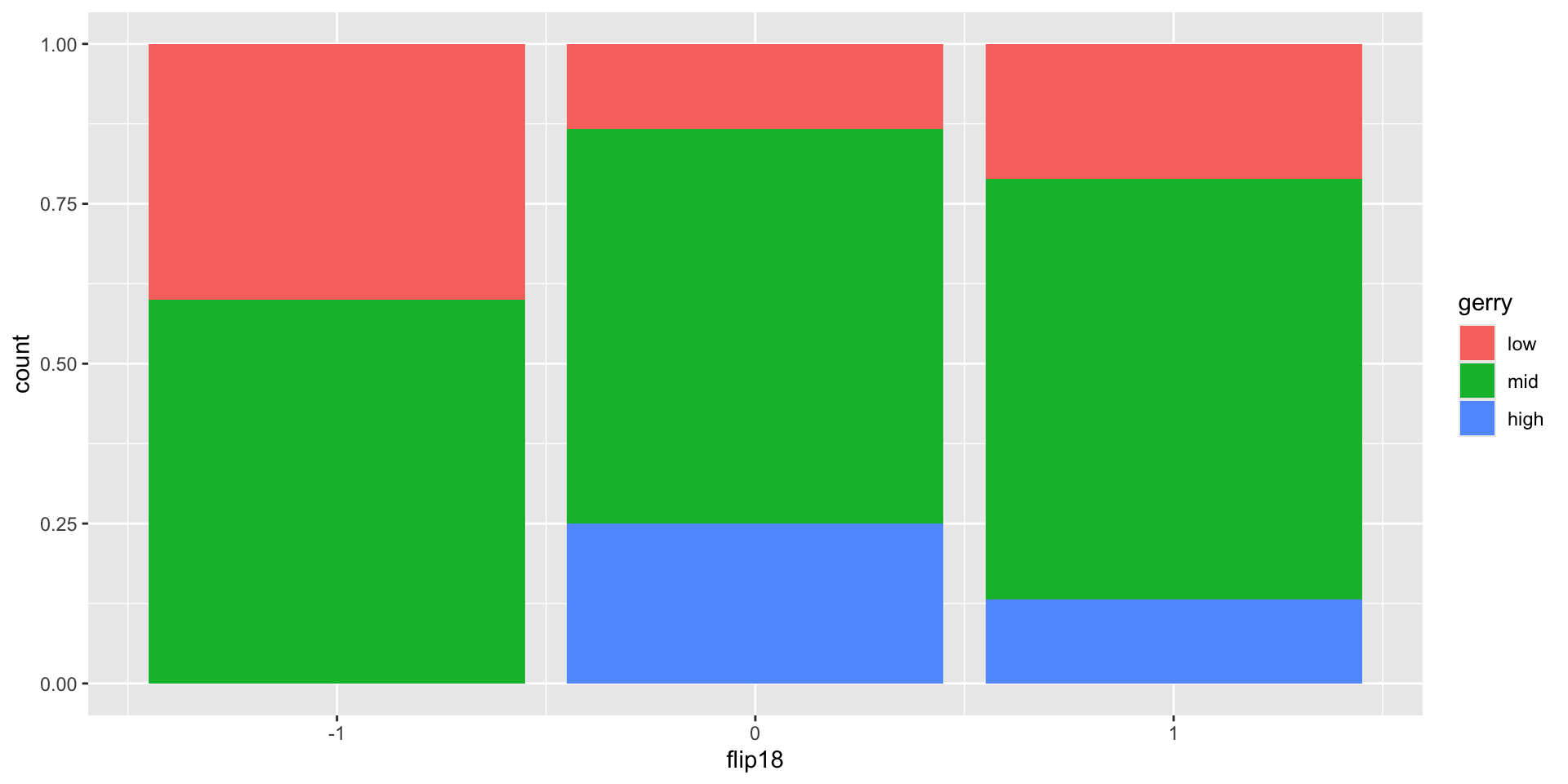
Is a Congressional District more likely to have high prevalence of gerrymandering if a Democrat was able to flip the seat in the 2018 election? Support your answer with a visualization as well as summary statistics.
Step 1
ggplot(gerrymander)
Step 2
Step 3
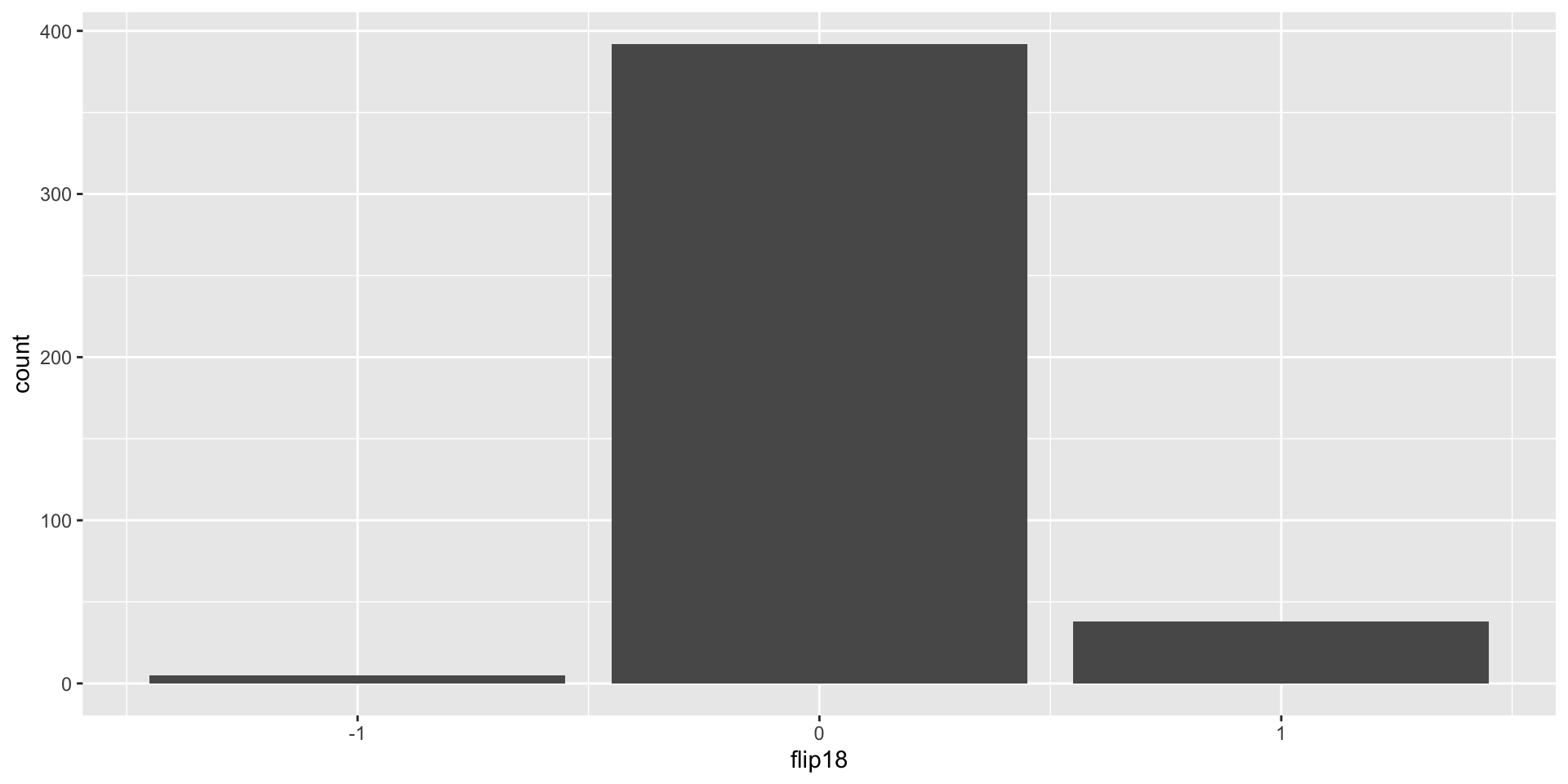
Step 4
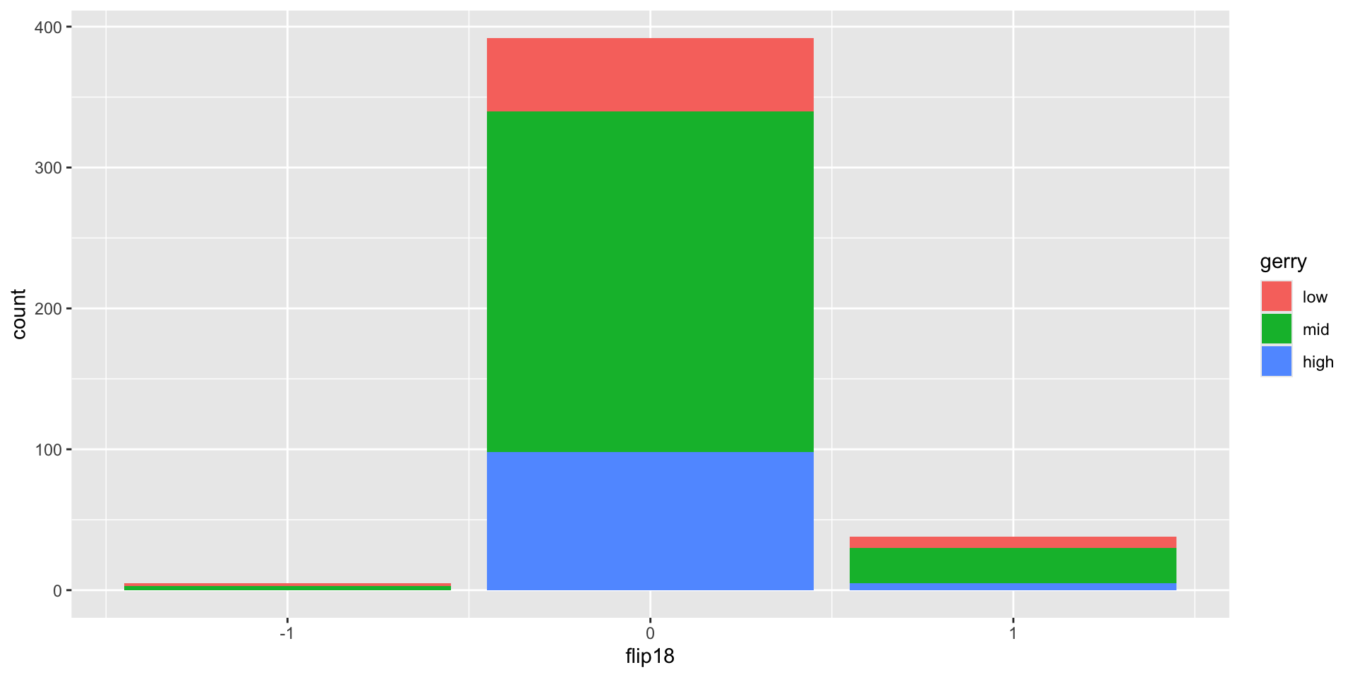
Step 5a
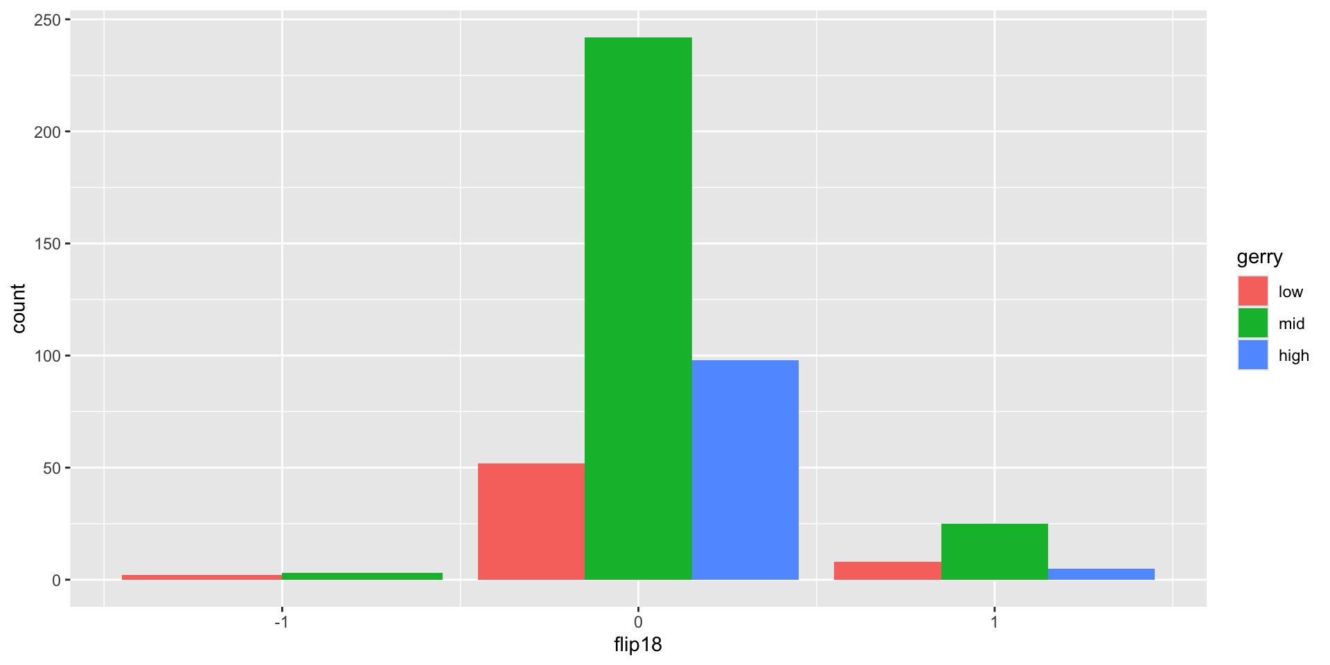
Step 5b
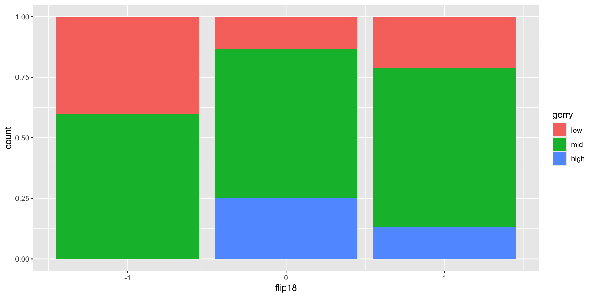
What’s the answer?
Is a Congressional District more likely to have high prevalence of gerrymandering if a Democrat was able to flip the seat in the 2018 election?
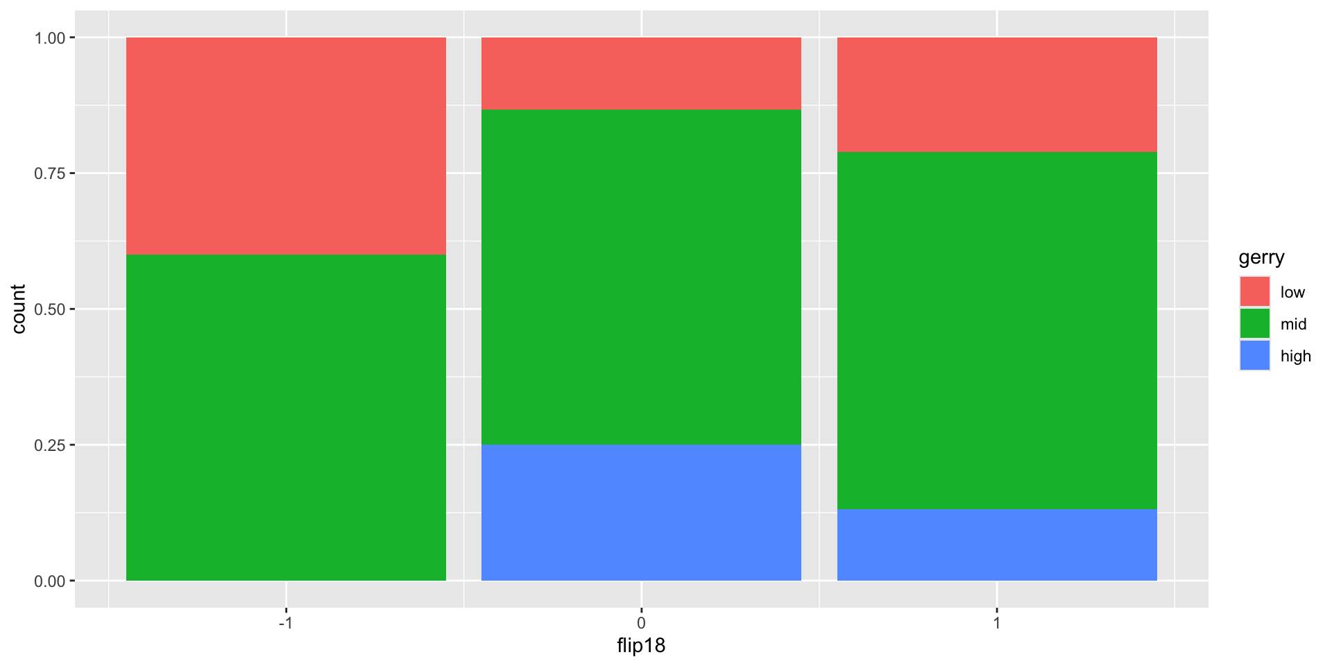
What are the actual numbers?
Is a Congressional District more likely to have high prevalence of gerrymandering if a Democrat was able to flip the seat in the 2018 election?
Step 1
gerrymander# A tibble: 435 × 12
district last_name first_name party16 clinton16 trump16 dem16 state party18
<chr> <chr> <chr> <chr> <dbl> <dbl> <dbl> <chr> <chr>
1 AK-AL Young Don R 37.6 52.8 0 AK R
2 AL-01 Byrne Bradley R 34.1 63.5 0 AL R
3 AL-02 Roby Martha R 33 64.9 0 AL R
4 AL-03 Rogers Mike D. R 32.3 65.3 0 AL R
5 AL-04 Aderholt Rob R 17.4 80.4 0 AL R
6 AL-05 Brooks Mo R 31.3 64.7 0 AL R
7 AL-06 Palmer Gary R 26.1 70.8 0 AL R
8 AL-07 Sewell Terri D 69.8 28.6 1 AL D
9 AR-01 Crawford Rick R 30.2 65 0 AR R
10 AR-02 Hill French R 41.7 52.4 0 AR R
# ℹ 425 more rows
# ℹ 3 more variables: dem18 <dbl>, flip18 <dbl>, gerry <fct>Step 2
gerrymander |>
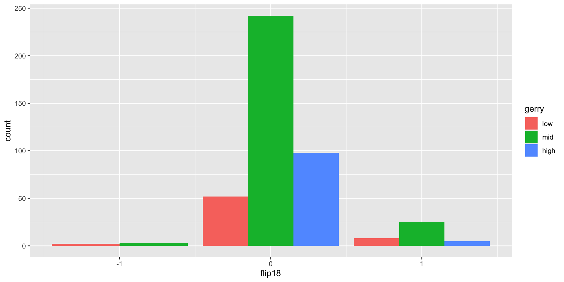
count(flip18, gerry)# A tibble: 8 × 3
flip18 gerry n
<dbl> <fct> <int>
1 -1 low 2
2 -1 mid 3
3 0 low 52
4 0 mid 242
5 0 high 98
6 1 low 8
7 1 mid 25
8 1 high 5Recall
The heights of these bars are the counts in the table:
Step 3
Step 4
The Full Monty
Is a Congressional District more likely to have high prevalence of gerrymandering if a Democrat flipped the seat in the 2018 election? (flip18 = 1: Democrat flipped the seat, 0: No flip, -1: Republican flipped the seat.)
New commands
countcreates a new data frame that tallies up the number of rows that fall into each bin;group_bysilently groups the rows according to bin, and all subsequent operations are done within group;-
mutateeither adds new columns that aren’t already there, or modifies existing columns.- we used it to add a
propcolumn that wasn’t there before; - because the table of counts is grouped, the proportions were computed within each level of
flip18.
- we used it to add a
That pesky pipe
We teach you to do this
You could do this instead
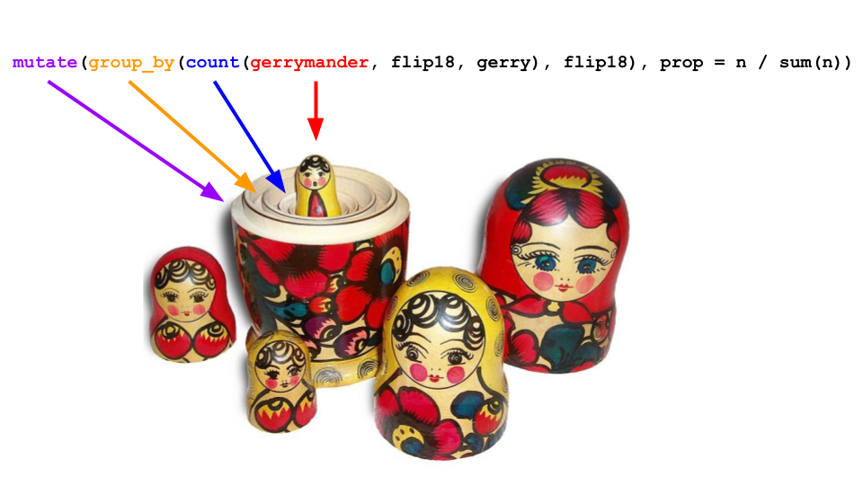
Technically equivalent. Gives the same result. Super hard to read:
Without the pipe
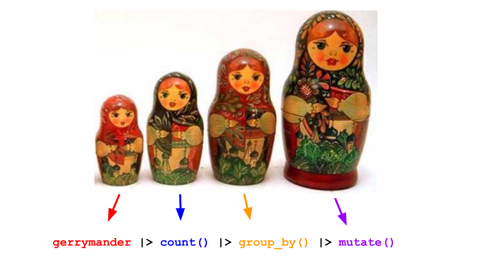
With the pipe
Drilling down:
group_by(),
summarize(),
count()
What does group_by() do?
What does group_by() do in the following pipeline?
What does group_by() do?
What does group_by() do in the following pipeline?
Let’s simplify!
What does group_by() do in the following pipeline?
Let’s simplify!
What does group_by() do in the following pipeline?
group_by()
it converts a data frame to a grouped data frame, where subsequent operations are performed once per group
ungroup()removes grouping
gerrymander |>
group_by(state)# A tibble: 435 × 12
# Groups: state [50]
district last_name first_name party16 clinton16 trump16 dem16 state party18
<chr> <chr> <chr> <chr> <dbl> <dbl> <dbl> <chr> <chr>
1 AK-AL Young Don R 37.6 52.8 0 AK R
2 AL-01 Byrne Bradley R 34.1 63.5 0 AL R
3 AL-02 Roby Martha R 33 64.9 0 AL R
4 AL-03 Rogers Mike D. R 32.3 65.3 0 AL R
5 AL-04 Aderholt Rob R 17.4 80.4 0 AL R
6 AL-05 Brooks Mo R 31.3 64.7 0 AL R
7 AL-06 Palmer Gary R 26.1 70.8 0 AL R
8 AL-07 Sewell Terri D 69.8 28.6 1 AL D
9 AR-01 Crawford Rick R 30.2 65 0 AR R
10 AR-02 Hill French R 41.7 52.4 0 AR R
# ℹ 425 more rows
# ℹ 3 more variables: dem18 <dbl>, flip18 <dbl>, gerry <fct>group_by()
it converts a data frame to a grouped data frame, where subsequent operations are performed once per group
ungroup()removes grouping
# A tibble: 435 × 12
   district last_name first_name party16 clinton16 trump16 dem16 state party18
   <chr>    <chr>     <chr>      <chr>       <dbl>   <dbl> <dbl> <chr> <chr>
 1 AK-AL    Young     Don        R            37.6    52.8     0 AK    R
 2 AL-01    Byrne     Bradley    R            34.1    63.5     0 AL    R
 3 AL-02    Roby      Martha     R            33      64.9     0 AL    R
 4 AL-03    Rogers    Mike D.    R            32.3    65.3     0 AL    R
 5 AL-04    Aderholt  Rob        R            17.4    80.4     0 AL    R
 6 AL-05    Brooks    Mo         R            31.3    64.7     0 AL    R
 7 AL-06    Palmer    Gary       R            26.1    70.8     0 AL    R
 8 AL-07    Sewell    Terri      D            69.8    28.6     1 AL    D
 9 AR-01    Crawford  Rick       R            30.2    65       0 AR    R
10 AR-02    Hill      French     R            41.7    52.4     0 AR    R
# ℹ 425 more rows
# ℹ 3 more variables: dem18 <dbl>, flip18 <dbl>, gerry <fct>group_by() |> summarize()
A common pipeline is group_by() and then summarize() to calculate summary statistics for each group:
gerrymander |>
group_by(state) |>
summarize(
mean_trump16 = mean(trump16),
median_trump16 = median(trump16)
)# A tibble: 50 × 3
state mean_trump16 median_trump16
<chr> <dbl> <dbl>
1 AK 52.8 52.8
2 AL 62.6 64.9
3 AR 60.9 63.0
4 AZ 46.9 47.7
5 CA 31.7 28.4
6 CO 43.6 41.3
7 CT 41.0 40.4
8 DE 41.9 41.9
9 FL 47.9 49.6
10 GA 51.3 56.6
# ℹ 40 more rowsgroup_by() |> summarize()
This pipeline can also be used to count number of observations for each group:
summarize()
... |>
  summarize(
    name_of_summary_statistic = summary_function(variable)
  )
. . .
Spot the difference
What’s the difference between the following two pipelines?
gerrymander |>
  count(state)
# A tibble: 50 × 2
state n
<chr> <int>
1 AK 1
2 AL 7
3 AR 4
4 AZ 9
5 CA 53
6 CO 7
7 CT 5
8 DE 1
9 FL 27
10 GA 14
# ℹ 40 more rowscount()
Count the number of observations in each level of variable(s)
Place the counts in a variable called
n
count() and sort
What does the following pipeline do? Rewrite it with count() instead.
count() and sort
What does the following pipeline do? Rewrite it with count() instead.
count() and sort
What does the following pipeline do? Rewrite it with count() instead.
gerrymander |>
  count(state, sort = TRUE)
# A tibble: 50 × 2
state n
<chr> <int>
1 CA 53
2 TX 36
3 FL 27
4 NY 27
5 IL 18
6 PA 18
7 OH 16
8 GA 14
9 MI 14
10 NC 13
# ℹ 40 more rowsSummary
“Science”?
- We call it “statistical science” or “data science,” but frankly it’s all much closer to art and rhetoric and storytelling;
- When you compress a data set down to pictures and summaries, you make countless choices about how to visualize, which summaries to inspect, how much detail to retain or discard, etc;
- A choice is good or bad insofar as a skeptical human audience finds it informative and persuasive.
Fine, but what dataviz should I use?
If you want to know where to begin, the number and type of variables typically narrows down the menu of options:
. . .
| Variable combo | Options for a first pass |
|---|---|
| 1 numerical | histogram, density, box plot, … |
| 1 categorical | bar chart, |
| 2 numerical | scatterplot |
| numerical/categorical | side-by-side boxes, stacked densities or histograms, … |
| 2 categorical | stacked bar plot |
. . .
For three or more variables, the human mind is limited, and you have to get creative (play with color, shape, texture, etc).
Computational themes
Every coding task in this class will be some combo of these two things:
. . .
Building cakes (ggplot) 
Stacking dolls (pipe |>) 
. . .
Master these, and everything will be coming up roses!
Where to now?
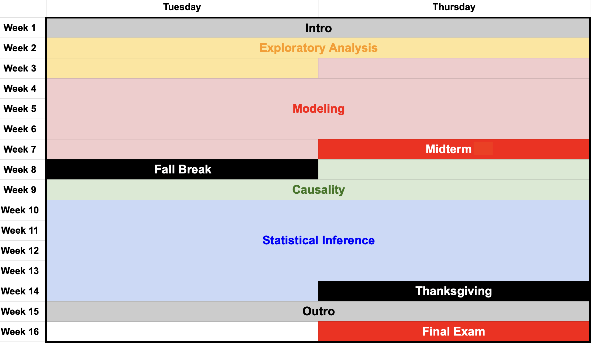
Where to now?
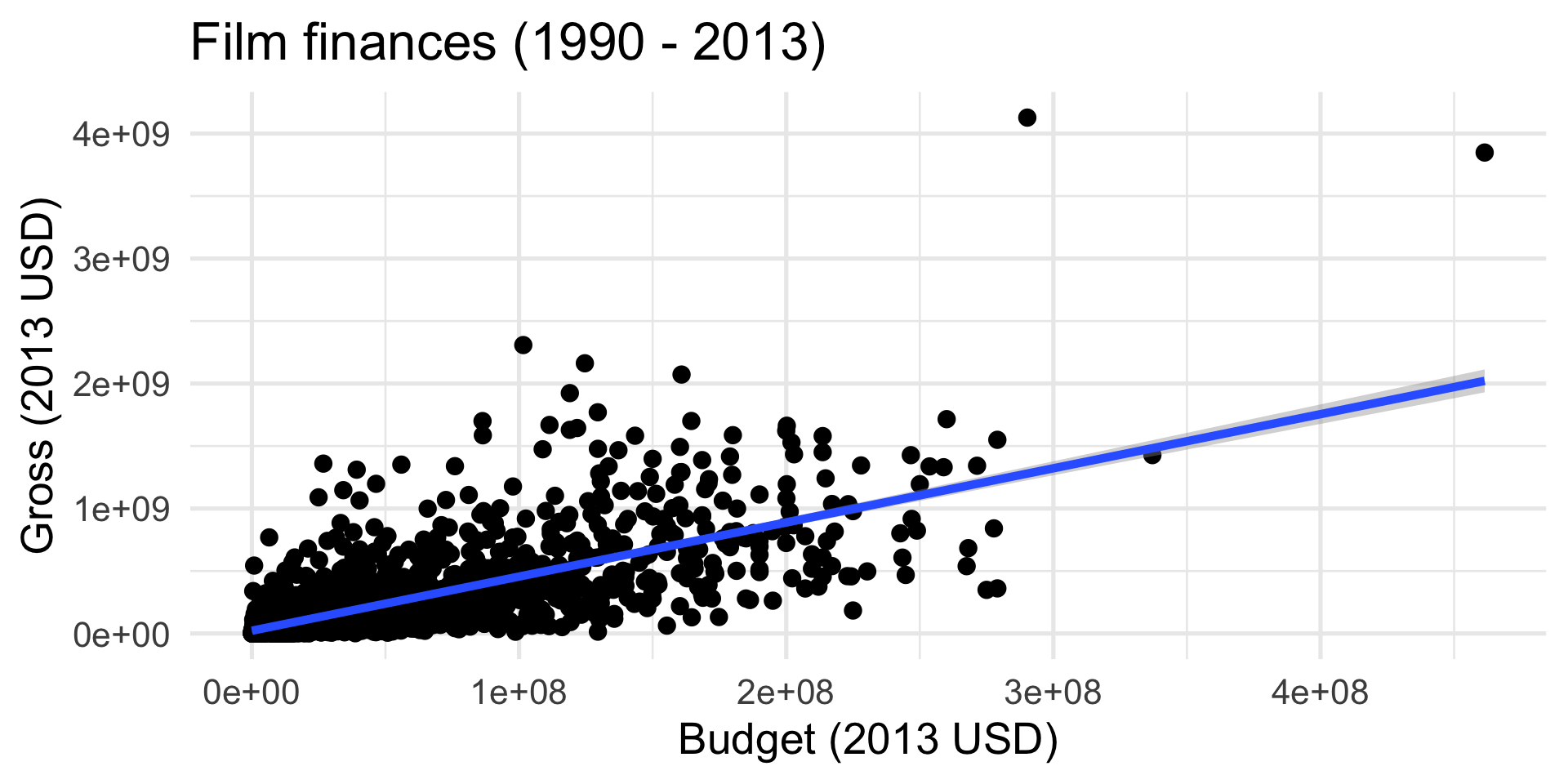
Where did the line come from? How was it drawn? How do you interpret it? How do you use it? What about more than two variables? What about categorical variables?