AE 6: building a spam filter
In this application exercise, we will
- Use logistic regression to fit a model for a binary response variable
- Fit a logistic regression model in R
- Use a logistic regression model for classification
To illustrate logistic regression, we will build a spam filter from email data.
The data come from incoming emails in David Diez’s Gmail account for the first three months of 2012. All personally identifiable information has been removed.
glimpse(email)Rows: 3,921
Columns: 21
$ spam <fct> 0, 0, 0, 0, 0, 0, 0, 0, 0, 0, 0, 0, 0, 0, 0, 0, 0, 0, 0, …
$ to_multiple <fct> 0, 0, 0, 0, 0, 0, 1, 1, 0, 0, 0, 0, 0, 0, 0, 0, 0, 0, 0, …
$ from <fct> 1, 1, 1, 1, 1, 1, 1, 1, 1, 1, 1, 1, 1, 1, 1, 1, 1, 1, 1, …
$ cc <int> 0, 0, 0, 0, 0, 0, 0, 1, 0, 0, 0, 1, 0, 1, 2, 1, 0, 2, 0, …
$ sent_email <fct> 0, 0, 0, 0, 0, 0, 1, 1, 0, 0, 1, 0, 0, 1, 0, 1, 0, 0, 1, …
$ time <dttm> 2012-01-01 01:16:41, 2012-01-01 02:03:59, 2012-01-01 11:…
$ image <dbl> 0, 0, 0, 0, 0, 0, 0, 1, 0, 0, 0, 0, 0, 0, 0, 0, 0, 0, 0, …
$ attach <dbl> 0, 0, 0, 0, 0, 0, 0, 1, 0, 0, 0, 0, 0, 0, 0, 0, 0, 0, 0, …
$ dollar <dbl> 0, 0, 4, 0, 0, 0, 0, 0, 0, 0, 0, 0, 0, 0, 2, 0, 5, 0, 0, …
$ winner <fct> no, no, no, no, no, no, no, no, no, no, no, no, no, no, n…
$ inherit <dbl> 0, 0, 1, 0, 0, 0, 0, 0, 0, 0, 0, 0, 0, 0, 0, 0, 0, 0, 0, …
$ viagra <dbl> 0, 0, 0, 0, 0, 0, 0, 0, 0, 0, 0, 0, 0, 0, 0, 0, 0, 0, 0, …
$ password <dbl> 0, 0, 0, 0, 2, 2, 0, 0, 0, 0, 0, 0, 0, 0, 0, 0, 1, 0, 0, …
$ num_char <dbl> 11.370, 10.504, 7.773, 13.256, 1.231, 1.091, 4.837, 7.421…
$ line_breaks <int> 202, 202, 192, 255, 29, 25, 193, 237, 69, 68, 25, 79, 191…
$ format <fct> 1, 1, 1, 1, 0, 0, 1, 1, 0, 1, 1, 0, 1, 1, 1, 1, 1, 1, 0, …
$ re_subj <fct> 0, 0, 0, 0, 0, 0, 0, 0, 0, 0, 0, 1, 0, 1, 1, 1, 0, 1, 1, …
$ exclaim_subj <dbl> 0, 0, 0, 0, 0, 0, 0, 0, 0, 0, 0, 0, 0, 0, 0, 0, 1, 0, 0, …
$ urgent_subj <fct> 0, 0, 0, 0, 0, 0, 0, 0, 0, 0, 0, 0, 0, 0, 0, 0, 0, 0, 0, …
$ exclaim_mess <dbl> 0, 1, 6, 48, 1, 1, 1, 18, 1, 0, 2, 1, 0, 10, 4, 10, 20, 0…
$ number <fct> big, small, small, small, none, none, big, small, small, …The variables we’ll use in this analysis are
-
spam: 1 if the email is spam, 0 otherwise -
exclaim_mess: The number of exclamation points in the email message
Goal: Use the number of exclamation points in an email to predict whether or not it is spam.
Exercises
Exercise 1
Let’s start with some exploratory analysis:
- Create a density plot to investigate the relationship between
spamandexclaim_mess.
ggplot(email, aes(x = exclaim_mess, fill = spam)) +
  geom_density()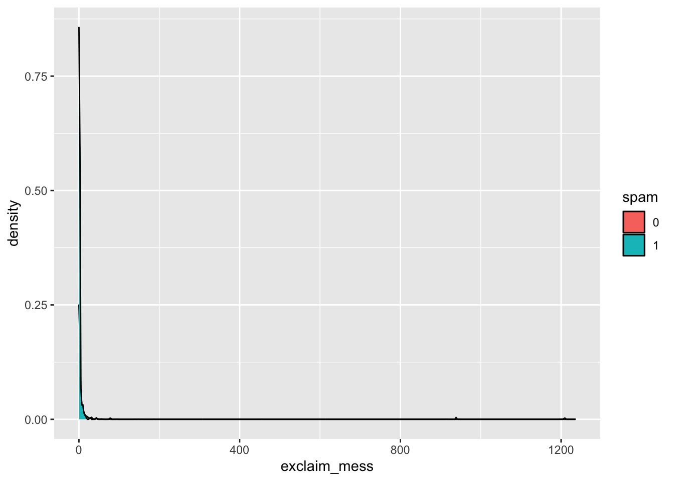
- Additionally, calculate the mean number of exclamation points for both spam and non-spam emails.
Exercise 2
Visualize a linear model fit for these data:
ggplot(email, aes(x = exclaim_mess, y = as.numeric(spam) - 1)) +
  geom_point() +
  geom_smooth(method = "lm") +
  labs(
    x = "# of exclamation marks in email",
    y = "e-mail type"
  ) +
  scale_y_continuous(breaks = c(0, 1),
                   labels = c("legit (0)", "spam (1)"))
`geom_smooth()` using formula = 'y ~ x'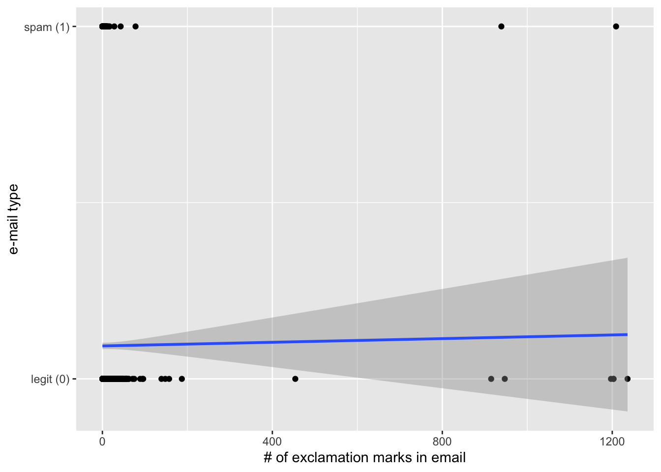
Is the linear model a good fit for the data? Why or why not?
Ans: Heavens no, are you kidding me?
Exercise 3
- Fit the logistic regression model using the number of exclamation points to predict the probability an email is spam:
log_fit <- logistic_reg() |>
  fit(spam ~ exclaim_mess, data = email)

tidy(log_fit)
# A tibble: 2 × 5
term estimate std.error statistic p.value
<chr> <dbl> <dbl> <dbl> <dbl>
1 (Intercept) -2.27 0.0553 -41.1 0
2 exclaim_mess 0.000272 0.000949 0.287 0.774- Add your estimates to the fitted equation below
\[\log\Big(\frac{\hat{p}}{1-\hat{p}}\Big) = -2.27 + 0.00027 \times exclaim\_mess\]
- Interpret stuff:
- For each additional exclamation mark, the model predicts that the odds of spam scale up by a factor of 1.00027 on average;
- The model predicts that an email with no exclamation marks has a 9.3% chance of being spam.
- How does the code above differ from previous code we’ve used to fit regression models?
Ans: linear_reg is changed to logistic_reg. Things are otherwise unchanged.
Exercise 4
- What is the probability the email is spam if it contains 10 exclamation points? Answer the question using the
predict()function.
# A tibble: 1 × 2
  .pred_0 .pred_1
    <dbl>   <dbl>
1 0.906 0.0937- A probability is nice, but we want an actual decision. Classify the darn email.
predict(log_fit, new_data = new_email, type = "class")# A tibble: 1 × 1
.pred_class
<fct>
1 0 The default behavior is to threshold the probabilities by 0.5.
Exercise 5
- Fit a model with all variables in the dataset as predictors.
log_fit2 <- logistic_reg() |>
  fit(spam ~ ., data = email)
Warning: glm.fit: fitted probabilities numerically 0 or 1 occurred- If you used this model to classify the emails in the dataset, how would it do? Use the fitted model to classify each email in the dataset, and then calculate the classification error rates (TP, TN, FP, FN).
log_aug <- augment(log_fit2, email)


log_aug |>
  count(spam, .pred_class) |>
  group_by(spam) |>
  mutate(p = n / sum(n))
# A tibble: 4 × 4
# Groups: spam [2]
spam .pred_class n p
<fct> <fct> <int> <dbl>
1 0 0 3521 0.991
2 0 1 33 0.00929
3 1 0 299 0.815
4 1 1 68 0.185 So:
- (True negative) 99.07%
- (False negative) 0.93%
- (False positive) 81.47%
- (True Positive) 18.53%
Exercise 6
If you change the classification threshold from the default (0.5) to something else, what happens to the classification accuracy of the model?
If we increase the threshold, we make it harder to classify an e-mail as spam, and so we have even fewer true positives, while the true negative rate stays put (it was already about as high as it could go):
log_aug |>
  mutate(
    .pred_class = if_else(.pred_1 >= 0.75, 1, 0)
  ) |>
  count(spam, .pred_class) |>
  group_by(spam) |>
  mutate(p = n / sum(n))
# A tibble: 4 × 4
# Groups: spam [2]
spam .pred_class n p
<fct> <dbl> <int> <dbl>
1 0 0 3544 0.997
2 0 1 10 0.00281
3 1 0 339 0.924
4 1 1 28 0.0763 If we decrease the threshold, we make it easier to classify an e-mail as spam, and so the true positive rate goes up by quite a bit, while the true negative rate only slips by a little bit. So perhaps the trade-off is worth it: