The language of models
Lecture 4
Modeling
Agenda
- What is a model?
- Why do we model?
- What is correlation?
Two main goals
Prediction / classification
Description / explanation
Prediction
Let’s drive a Tesla!
Description
Leisure, commute, physical activity and BP
Byambasukh, Oyuntugs, Harold Snieder, and Eva Corpeleijn. “Relation between leisure time, commuting, and occupational physical activity with blood pressure in 125 402 adults: the lifelines cohort.” Journal of the American Heart Association 9.4 (2020): e014313.
Leisure, commute, physical activity and BP
Goal: To investigate the associations of different domains of daily‐life physical activity, such as commuting, leisure‐time, and occupational, with BP level and the risk of having hypertension.
Leisure, commute, physical activity and BP
Goal: To investigate the associations of different domains of daily-life physical activity, such as commuting, leisure-time, and occupational, with BP level and the risk of having hypertension.
Methods and Results: In the population-based Lifelines cohort (N=125,402), MVPA was assessed by the Short Questionnaire to Assess Health-Enhancing Physical Activity, a validated questionnaire in different domains such as commuting, leisure-time, and occupational PA.
Leisure, commute, physical activity and BP
Goal: To investigate the associations of different domains of daily-life physical activity, such as commuting, leisure-time, and occupational, with BP level and the risk of having hypertension.
Methods and Results: In the population-based Lifelines cohort (N=125,402), MVPA was assessed by the Short Questionnaire to Assess Health-Enhancing Physical Activity, a validated questionnaire in different domains such as commuting, leisure-time, and occupational PA. Commuting-and-leisure-time MVPA was associated with BP in a dose-dependent manner.
Leisure, commute, physical activity and BP
Goal: To investigate the associations of different domains of daily-life physical activity, such as commuting, leisure-time, and occupational, with BP level and the risk of having hypertension.
Methods and Results: In the population-based Lifelines cohort (N=125,402), MVPA was assessed by the Short Questionnaire to Assess Health-Enhancing Physical Activity, a validated questionnaire in different domains such as commuting, leisure-time, and occupational PA. Commuting-and-leisure-time MVPA was associated with BP in a dose-dependent manner. β Coefficients (95% CI) from linear regression analyses were −1.64 (−2.03 to −1.24), −2.29 (−2.68 to −1.90), and −2.90 (−3.29 to −2.50) mm Hg systolic BP for the low, middle, and highest tertile of MVPA compared with “No MVPA” as the reference group after adjusting for age, sex, education, smoking and alcohol use. Further adjustment for body mass index attenuated the associations by 30% to 50%, but more MVPA remained significantly associated with lower BP and lower risk of hypertension. This association was age dependent. β Coefficients (95% CI) for the highest tertiles of commuting-and-leisure-time MVPA were −1.67 (−2.20 to −1.15), −3.39 (−3.94 to −2.82) and −4.64 (−6.15 to −3.14) mm Hg systolic BP in adults <40, 40 to 60, and >60 years, respectively.
Leisure, commute, physical activity and BP
Goal: To investigate the associations of different domains of daily-life physical activity, such as commuting, leisure-time, and occupational, with BP level and the risk of having hypertension.
Methods and Results: In the population-based Lifelines cohort (N=125,402), MVPA was assessed by the Short Questionnaire to Assess Health-Enhancing Physical Activity, a validated questionnaire in different domains such as commuting, leisure-time, and occupational PA. Commuting-and-leisure-time MVPA was associated with BP in a dose-dependent manner. β Coefficients (95% CI) from linear regression analyses were −1.64 (−2.03 to −1.24), −2.29 (−2.68 to −1.90), and −2.90 (−3.29 to −2.50) mm Hg systolic BP for the low, middle, and highest tertile of MVPA compared with “No MVPA” as the reference group after adjusting for age, sex, education, smoking and alcohol use. Further adjustment for body mass index attenuated the associations by 30% to 50%, but more MVPA remained significantly associated with lower BP and lower risk of hypertension. This association was age dependent. β Coefficients (95% CI) for the highest tertiles of commuting-and-leisure-time MVPA were −1.67 (−2.20 to −1.15), −3.39 (−3.94 to −2.82) and −4.64 (−6.15 to −3.14) mm Hg systolic BP in adults <40, 40 to 60, and >60 years, respectively.
Conclusions: Higher commuting and leisure-time but not occupational MVPA were significantly associated with lower BP and lower hypertension risk at all ages, but these associations were stronger in older adults.
Some themes
- A model takes inputs and generates predictions;
- A model is statistical if it delivers uncertainty quantification for the predictions and conclusions;
- Model outputs are just like any other summary. It’s just our best guess;
- All models are wrong, but some are useful;
- Beware the reflex to interpret the model as “input causes output.” Maybe. Maybe not.
Let’s go
Modeling cars
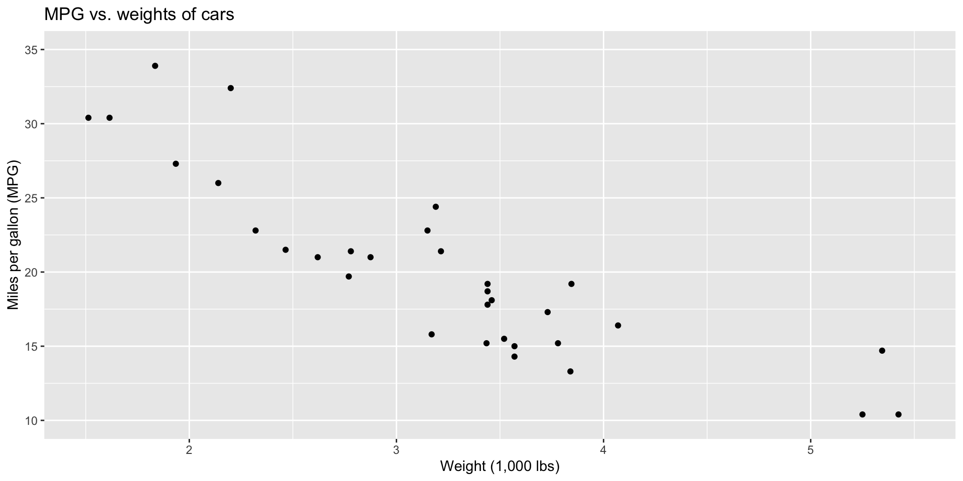
- What is the relationship between cars’ weights and their mileage?
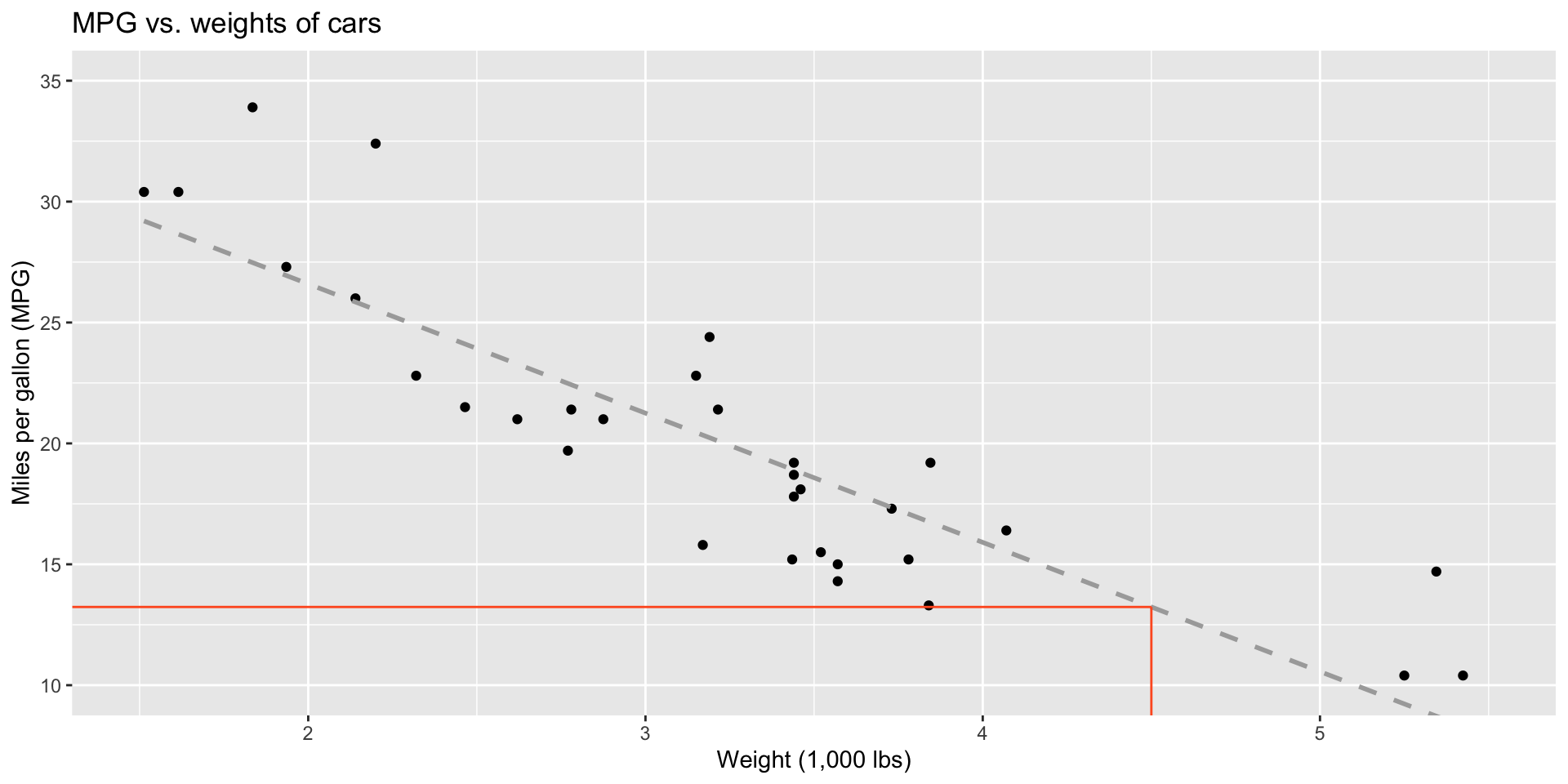
- What is your best guess for a car’s MPG that weighs 4,500 pounds?
Modelling cars
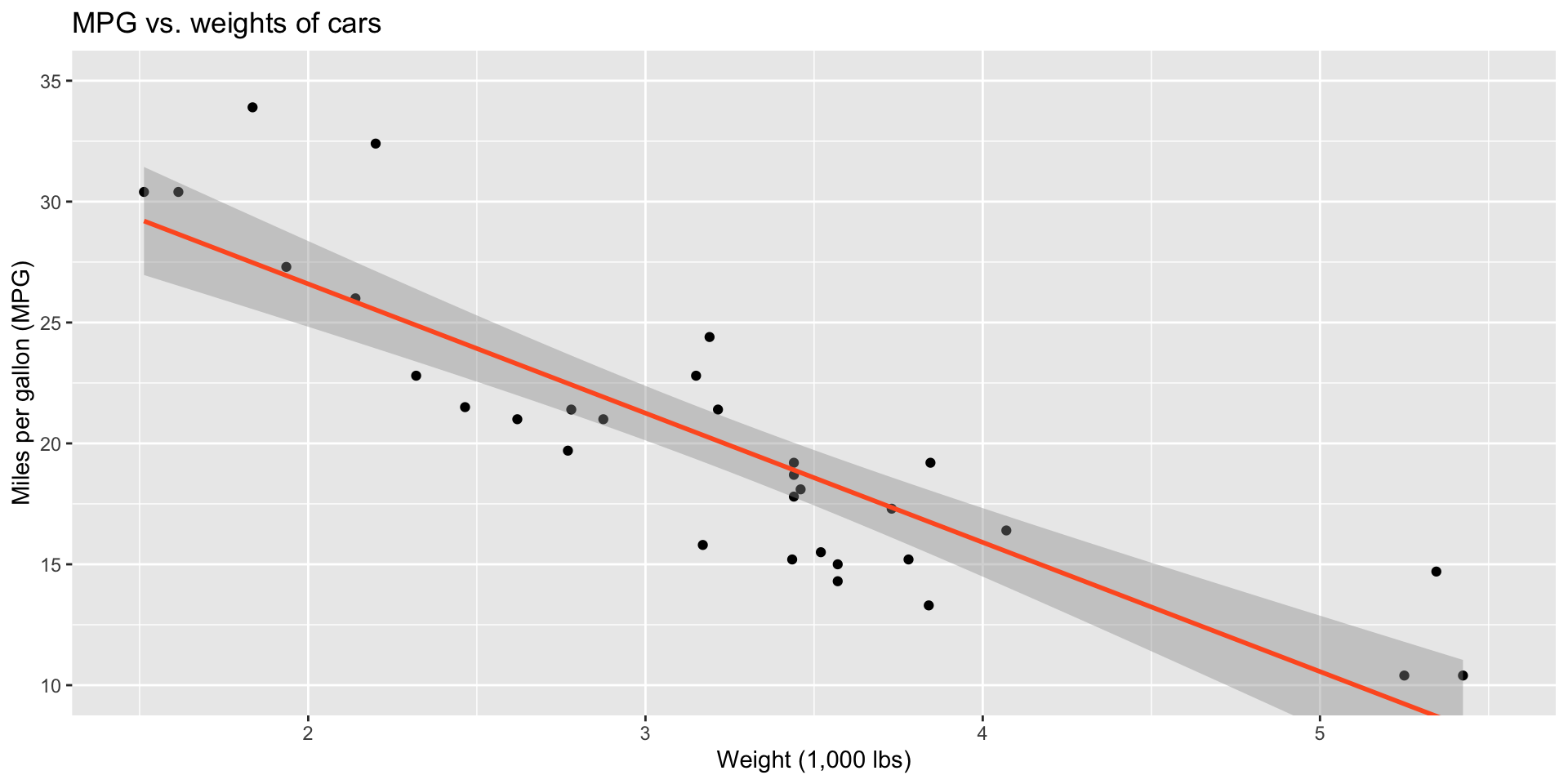
Describe: What is the relationship between cars’ weights and their mileage?
Modelling cars
Predict: What is your best guess for a car’s MPG that weighs 4,500 pounds?
Modelling
- Use models to explain the relationship between variables and to make predictions
- For now we will focus on linear models (but there are many many other types of models too!)
What is a line?
But on a plot…
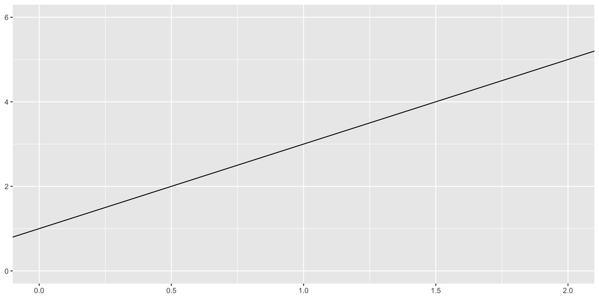
But in math terms…
\[ \begin{aligned} y &= mx + b \\ \text{Output}&=\text{Slope}\times \text{Input} + \text{Intercept} \end{aligned} \]
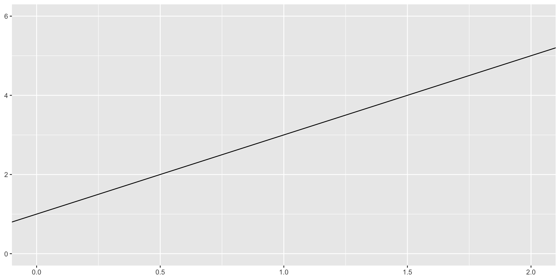
Modelling vocabulary
- Predictor (explanatory variable)
- Outcome (response variable)
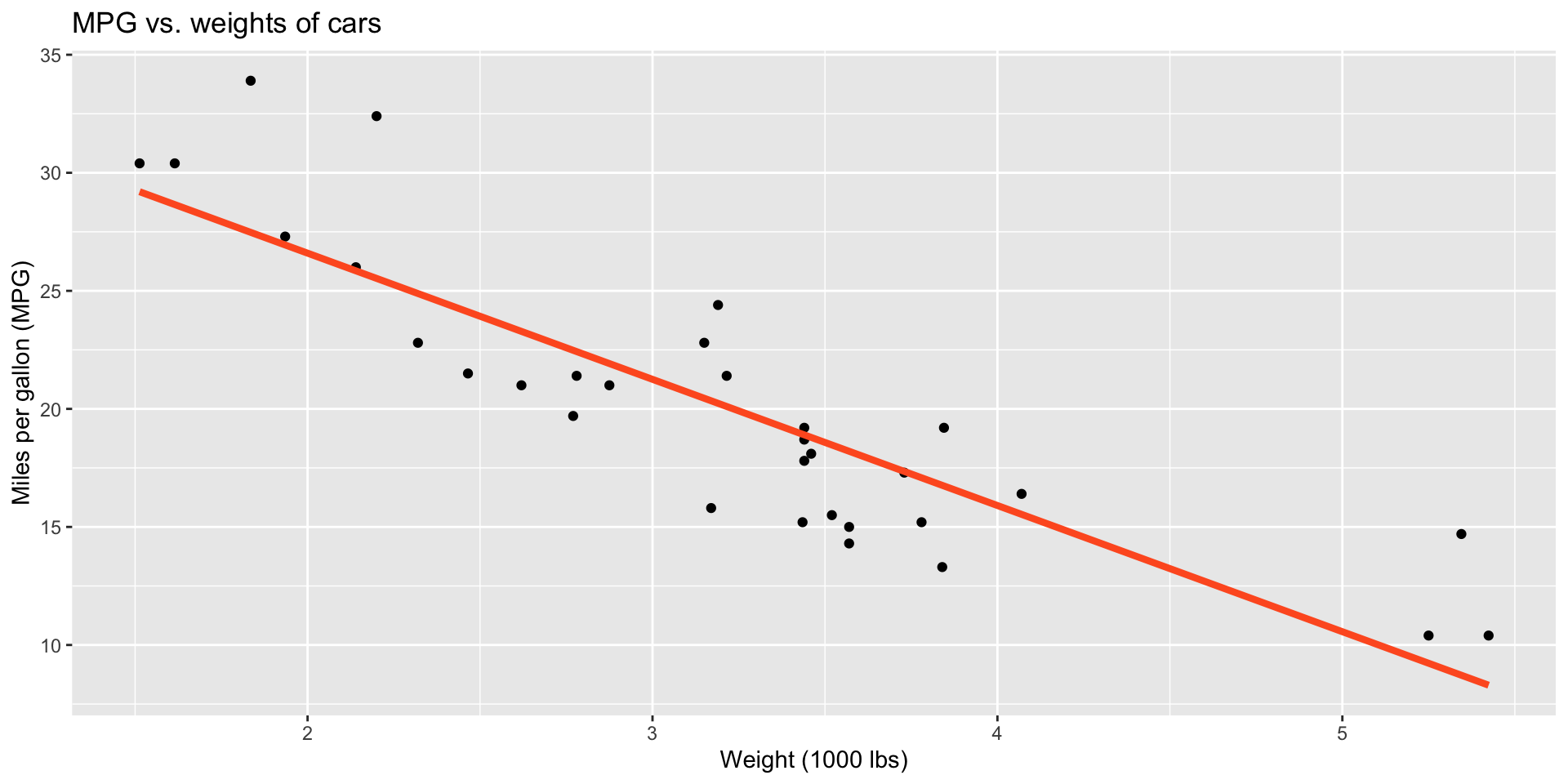
- Regression line
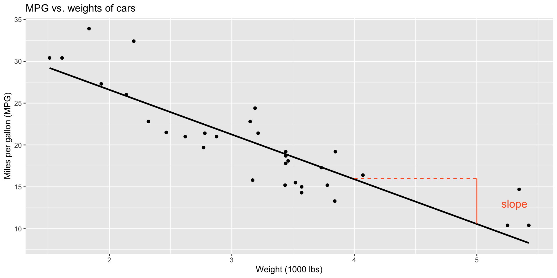
- Slope
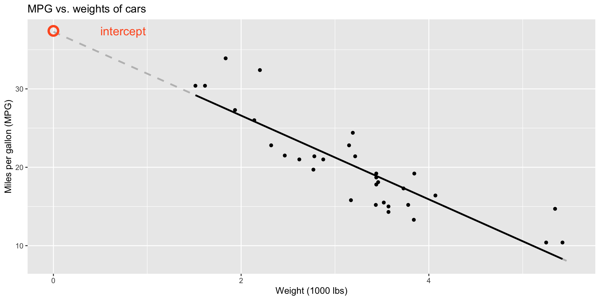
- Intercept
- Correlation
Predictor (explanatory variable)
| mpg | wt |
|---|---|
| 21 | 2.62 |
| 21 | 2.875 |
| 22.8 | 2.32 |
| 21.4 | 3.215 |
| 18.7 | 3.44 |
| 18.1 | 3.46 |
| ... | ... |
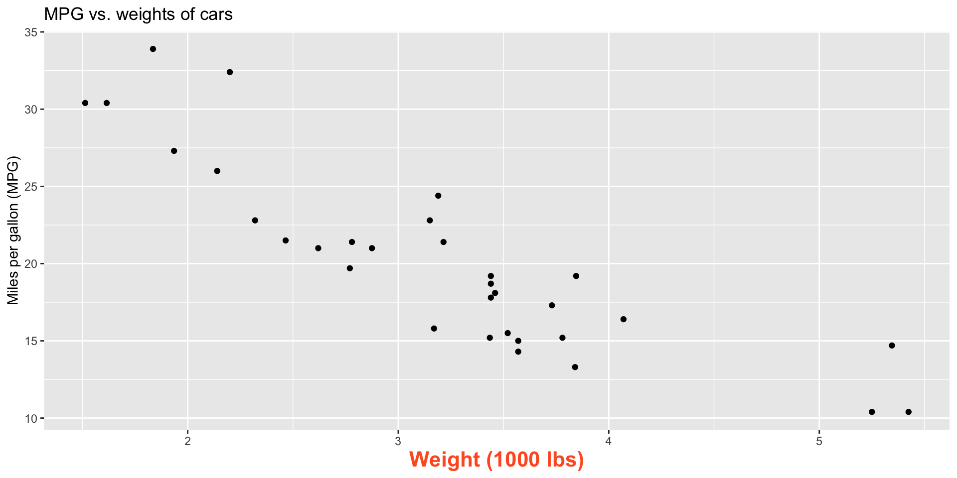
Outcome (response variable)
| mpg | wt |
|---|---|
| 21 | 2.62 |
| 21 | 2.875 |
| 22.8 | 2.32 |
| 21.4 | 3.215 |
| 18.7 | 3.44 |
| 18.1 | 3.46 |
| ... | ... |
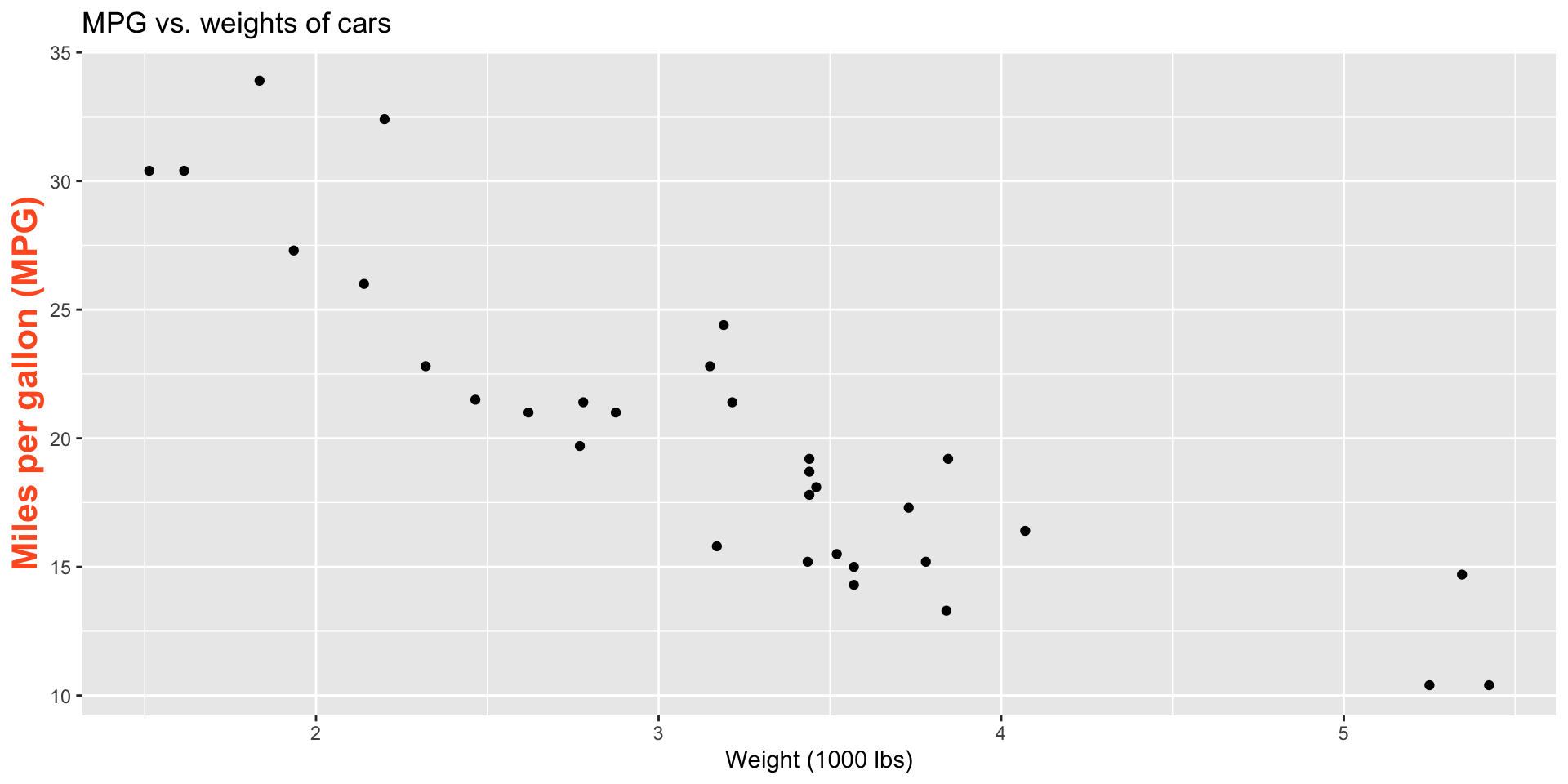
Regression line
Regression line: slope
Regression line: intercept
Correlation
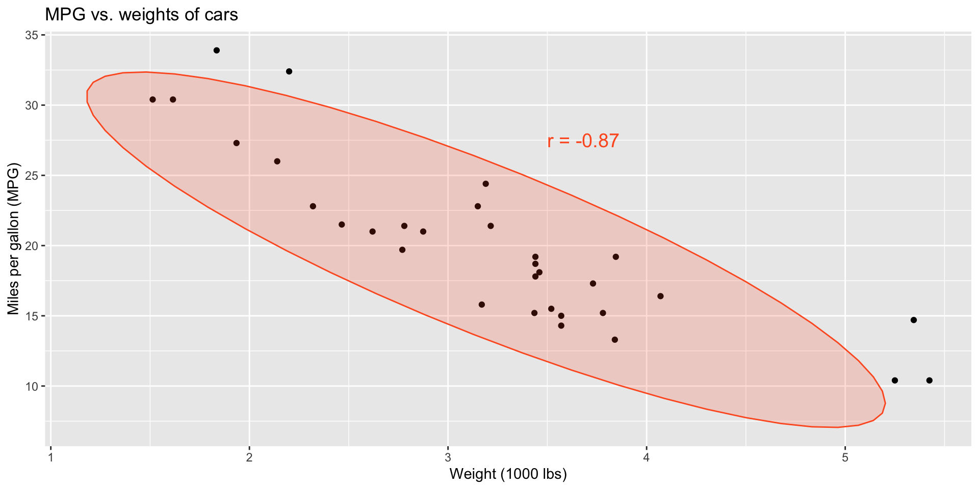
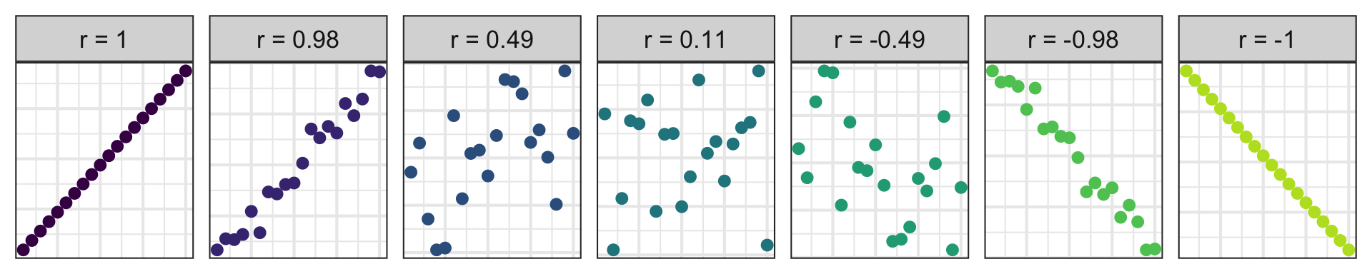
Correlation
- Measures the strength and direction of the linear association between two numerical variables;
- Tells you how tightly the points cluster around a straight line;
- Ranges between -1 and 1;
- Same sign as the slope.
New command: cor
df# A tibble: 20 × 2
x y
<int> <dbl>
1 1 -34.8
2 2 -184.
3 3 -154.
4 4 -326.
5 5 -76.6
6 6 -213.
7 7 -331.
8 8 511.
9 9 288.
10 10 46.0
11 11 -182.
12 12 265.
13 13 308.
14 14 118.
15 15 -435.
16 16 110.
17 17 392.
18 18 250.
19 19 287.
20 20 246. df |>
summarize(
r = cor(x, y)
)# A tibble: 1 × 1
r
<dbl>
1 0.501Practice!
https://www.rossmanchance.com/applets/2021/guesscorrelation/GuessCorrelation.html
. . .
(Just the sort of pain in the ass visual intuition crap that JZ is liable to put on an exam.)
Visualizing the model
ggplot(mtcars, aes(x = wt, y = mpg)) +
  geom_point()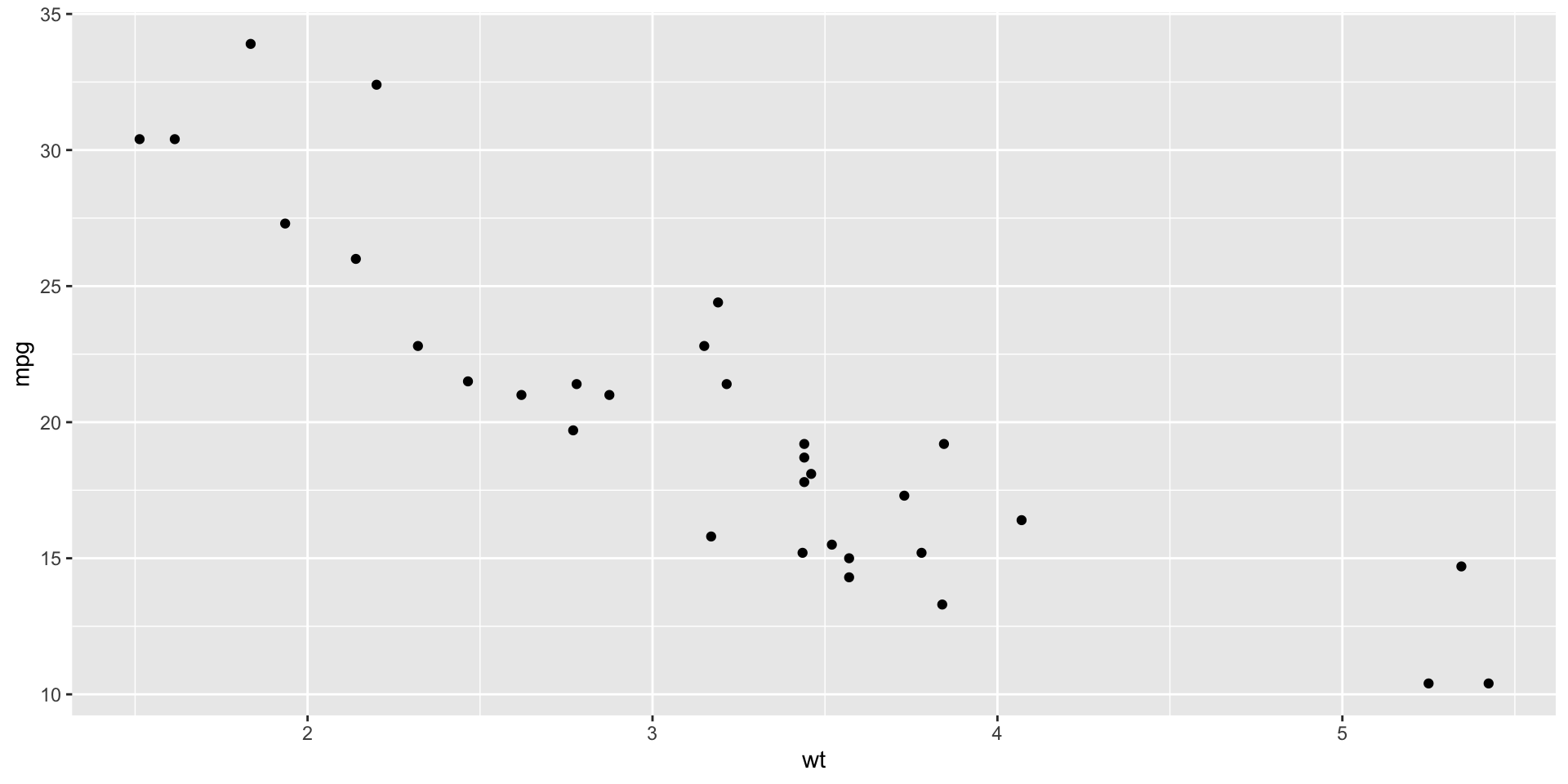
Visualizing the model
ggplot(mtcars, aes(x = wt, y = mpg)) +
  geom_point() +
  geom_smooth()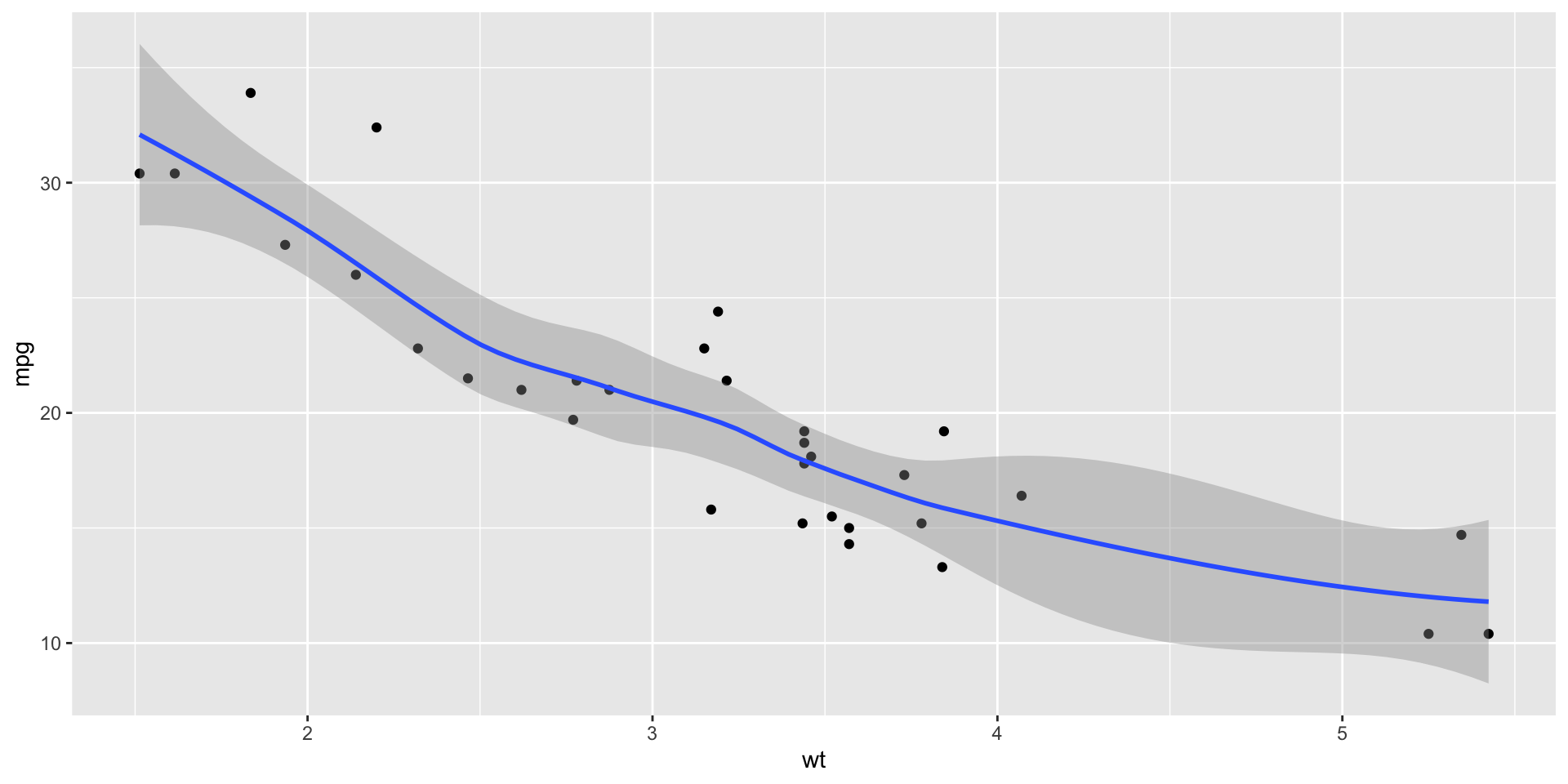
Visualizing the model
ggplot(mtcars, aes(x = wt, y = mpg)) +
  geom_point() +
  geom_smooth(method = "loess")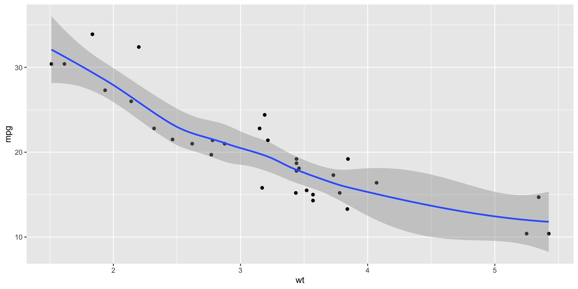
Visualizing the model
ggplot(mtcars, aes(x = wt, y = mpg)) +
  geom_point() +
  geom_smooth(method = "lm")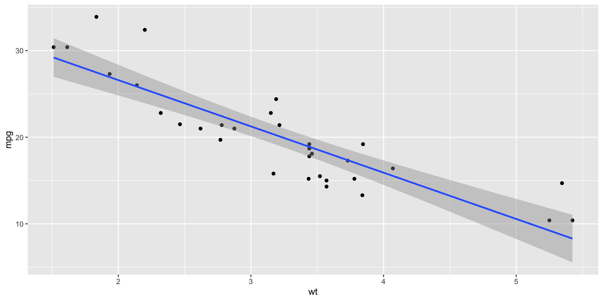
Don’t forget: Always Be Visualizing!
Anscombe’s Quartet
Dataset I
    x     y
1  10  8.04
2   8  6.95
3  13  7.58
4   9  8.81
5  11  8.33
6  14  9.96
7   6  7.24
8   4  4.26
9  12 10.84
10  7  4.82
11  5  5.68
Dataset II
    x    y
1  10 9.14
2   8 8.14
3  13 8.74
4   9 8.77
5  11 9.26
6  14 8.10
7   6 6.13
8   4 3.10
9  12 9.13
10  7 7.26
11  5 4.74
Dataset III
    x     y
1  10  7.46
2   8  6.77
3  13 12.74
4   9  7.11
5  11  7.81
6  14  8.84
7   6  6.08
8   4  5.39
9  12  8.15
10  7  6.42
11  5  5.73
Dataset IV
    x     y
1   8  6.58
2   8  5.76
3   8  7.71
4   8  8.84
5   8  8.47
6   8  7.04
7   8  5.25
8  19 12.50
9   8  5.56
10  8  7.91
11  8  6.89
Very different
ggplot(anscombe_tidy, aes(x, y)) +
  geom_point() +
facet_wrap(~ set) 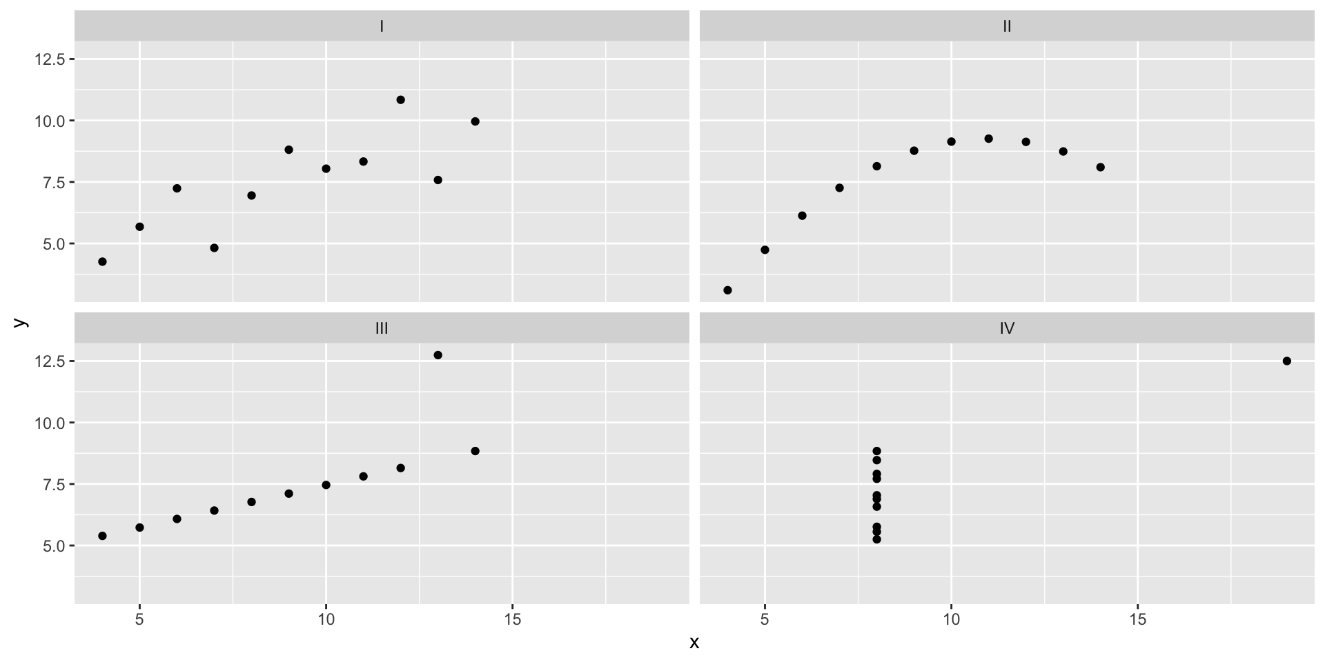
But it’s the same line…
ggplot(anscombe_tidy, aes(x, y)) +
  geom_point() +
  facet_wrap(~ set) +
  geom_smooth(method = "lm", se = FALSE)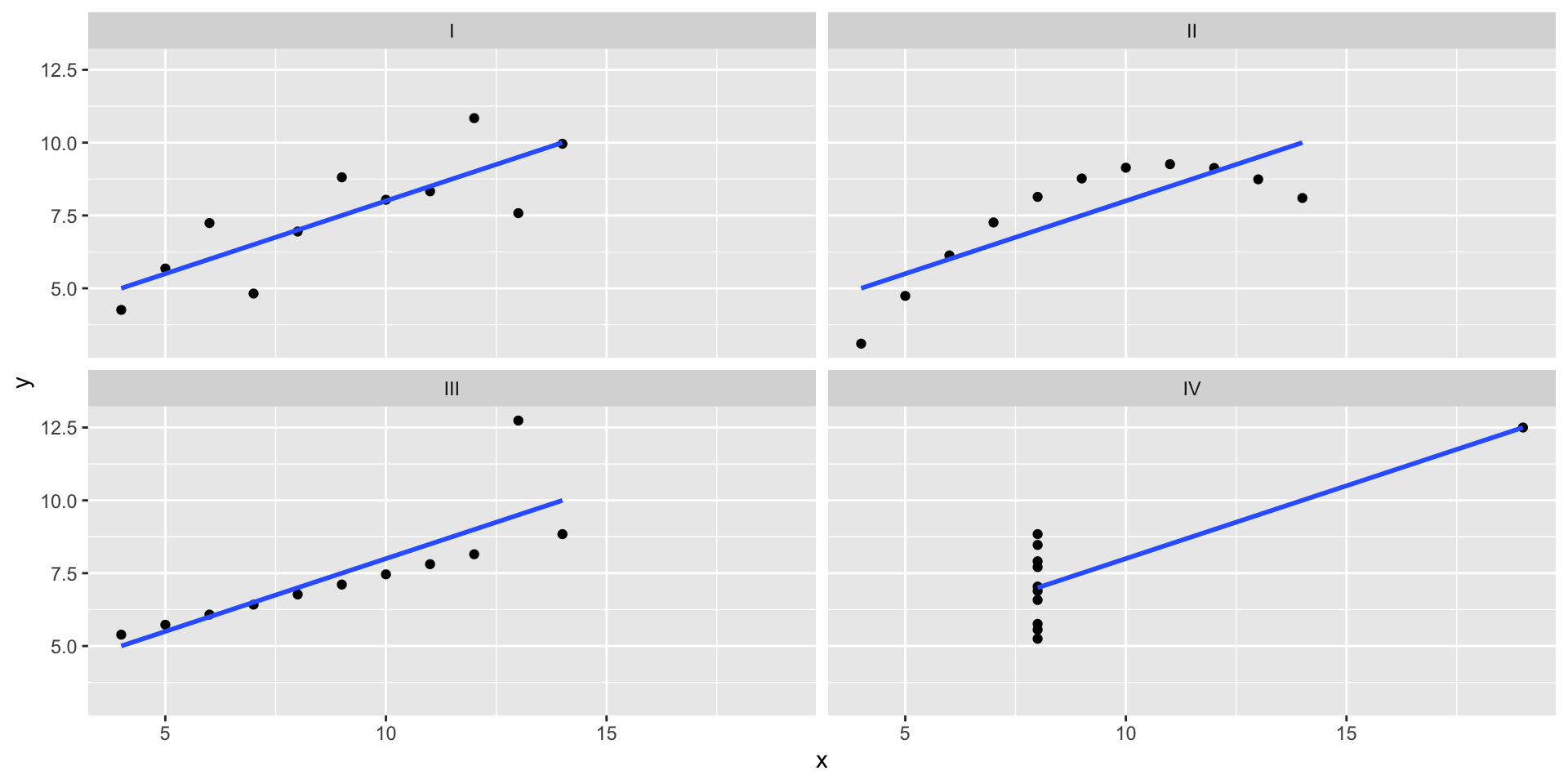
…and the same summary statistics.
anscombe_tidy |>
  group_by(set) |>
  summarize(
    xbar = mean(x),
    ybar = mean(y),
    sx = sd(x),
    sy = sd(y),
    r = cor(x, y)
  )
# A tibble: 4 × 6
set xbar ybar sx sy r
<chr> <dbl> <dbl> <dbl> <dbl> <dbl>
1 I 9 7.50 3.32 2.03 0.816
2 II 9 7.50 3.32 2.03 0.816
3 III 9 7.5 3.32 2.03 0.816
4 IV 9 7.50 3.32 2.03 0.817New commands introduced today
In base R:
-
cor: compute correlation between two numerical variables;
In ggplot2:
-
geom_smooth: add model fit to scatterplot;
In the new package tidymodels:
-
linear_regandfit: estimate linear model; -
tidy: cute lil’ summary table of model output -
predict: use estimated model to predict.