Inference with the normal distribution

Lecture 17

John Zito

Duke University
STA 101 Fall 2026

2026-11-03

The story so far

Our statistical problem

We want to understand how two numerical variables $X$ and $Y$ are related;
We do so through the lens of this model:

\[ Y=\beta_0+\beta_1X+\varepsilon. \]
$\beta_1$ describes the relationship, and we want to know what it is;
Using a messy, meager, incomplete, imperfect sample of data, we construct our best guess:

\[ \widehat{Y}=b_0+b_1X. \]
$b_1$ is our point estimate of $\beta_1$. How reliable is it?

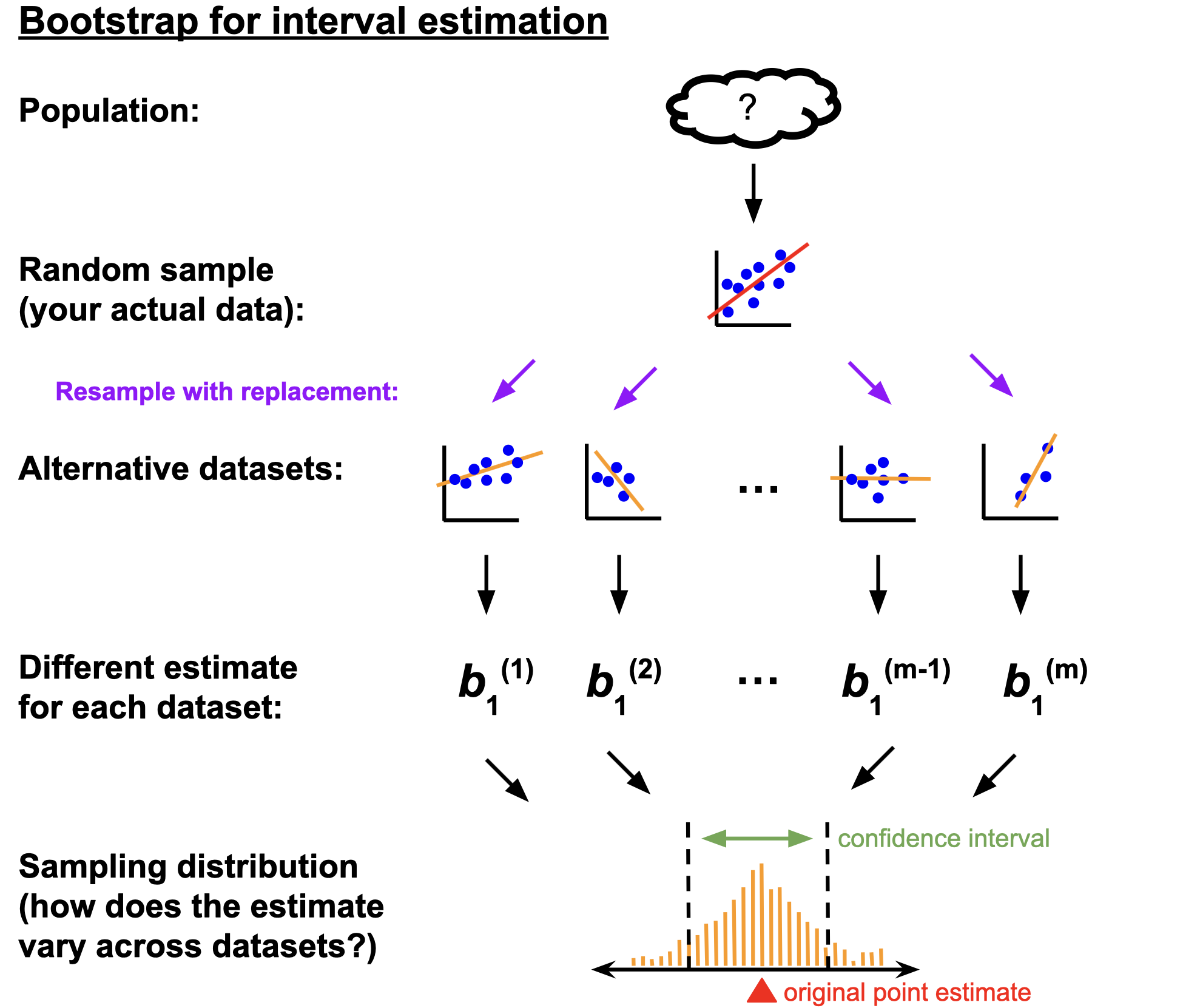
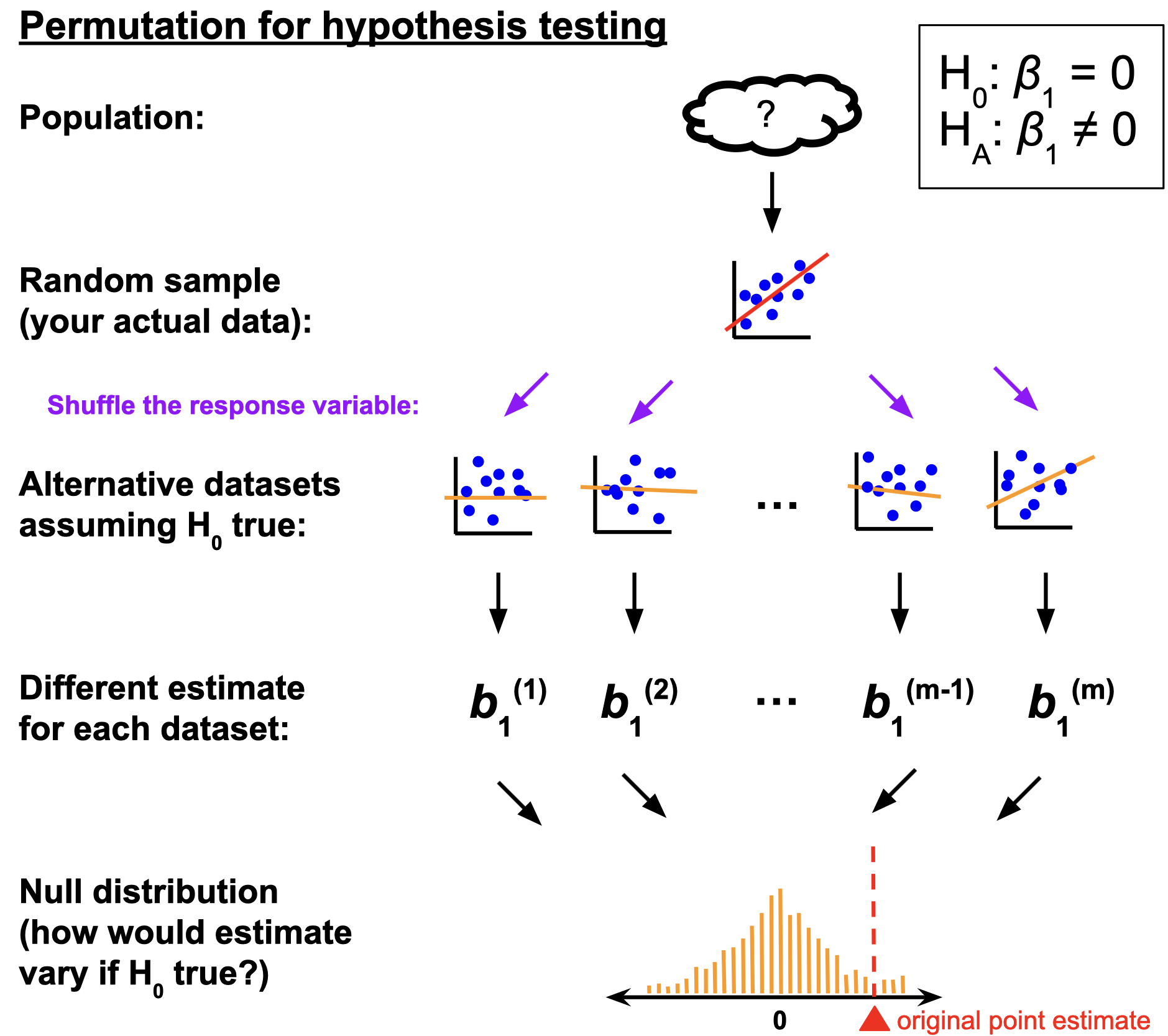
Grand summary from last time

Pay close attention to the similarities and differences:

The main ideas

In statistics, we quantify uncertainty with distributions:

The sampling distribution describes how an estimate would vary across alternative datasets;
- the spread of this distribution communicates uncertainty/reliability;
- high probability regions provide a range of likely values (confidence interval);
The null distribution describes how an estimate would vary across alternative datasets if the null hypothesis happened to be true;
- compare this to the actual point estimate to quantify the strength of evidence for competing claims.

We must approximate!

Literally collecting new, alternative datasets is costly and impractical (if it was so easy, we would have made our original sample size larger in the first place);
We fake it with simulation (bootstrapping or permutation) and approximate the sampling and null distributions with histograms;
Next, we explore a set of pencil-and-paper mathematical techniques for approximating these distributions.

(This is where things start to resemble AP Stats)

Recall this example

Recall the openintro::loans_full_schema data frame:

10000 rows;
each row is an approved loan applicant;
the columns contain financial info about that person, including…
- annual income (in log $);
- amount of non-mortgage debt outstanding (in log $).
What is the relationship between these two variables?

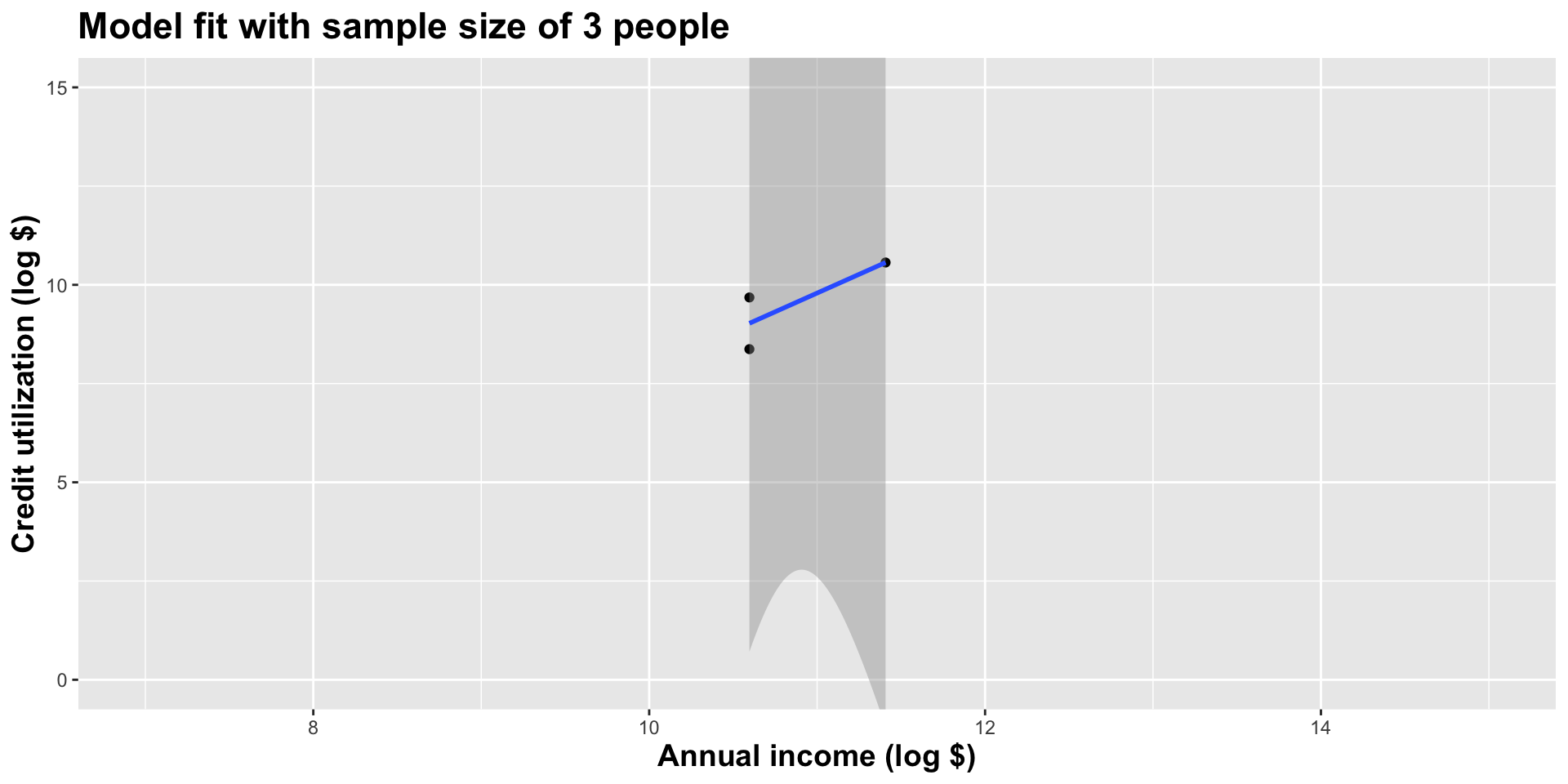
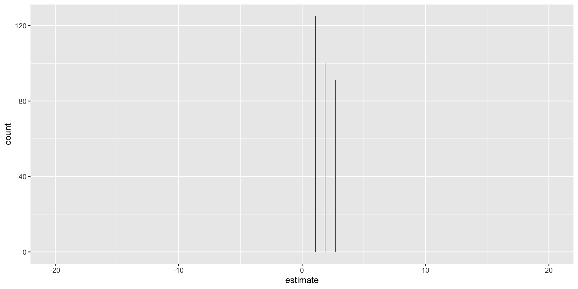
Model fit with three observations

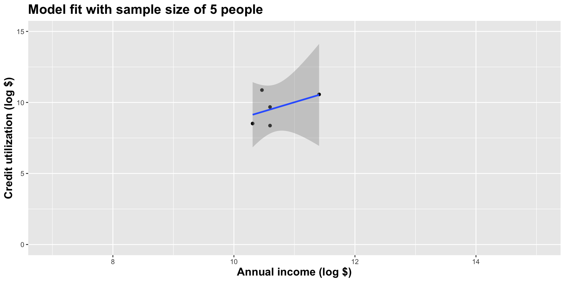
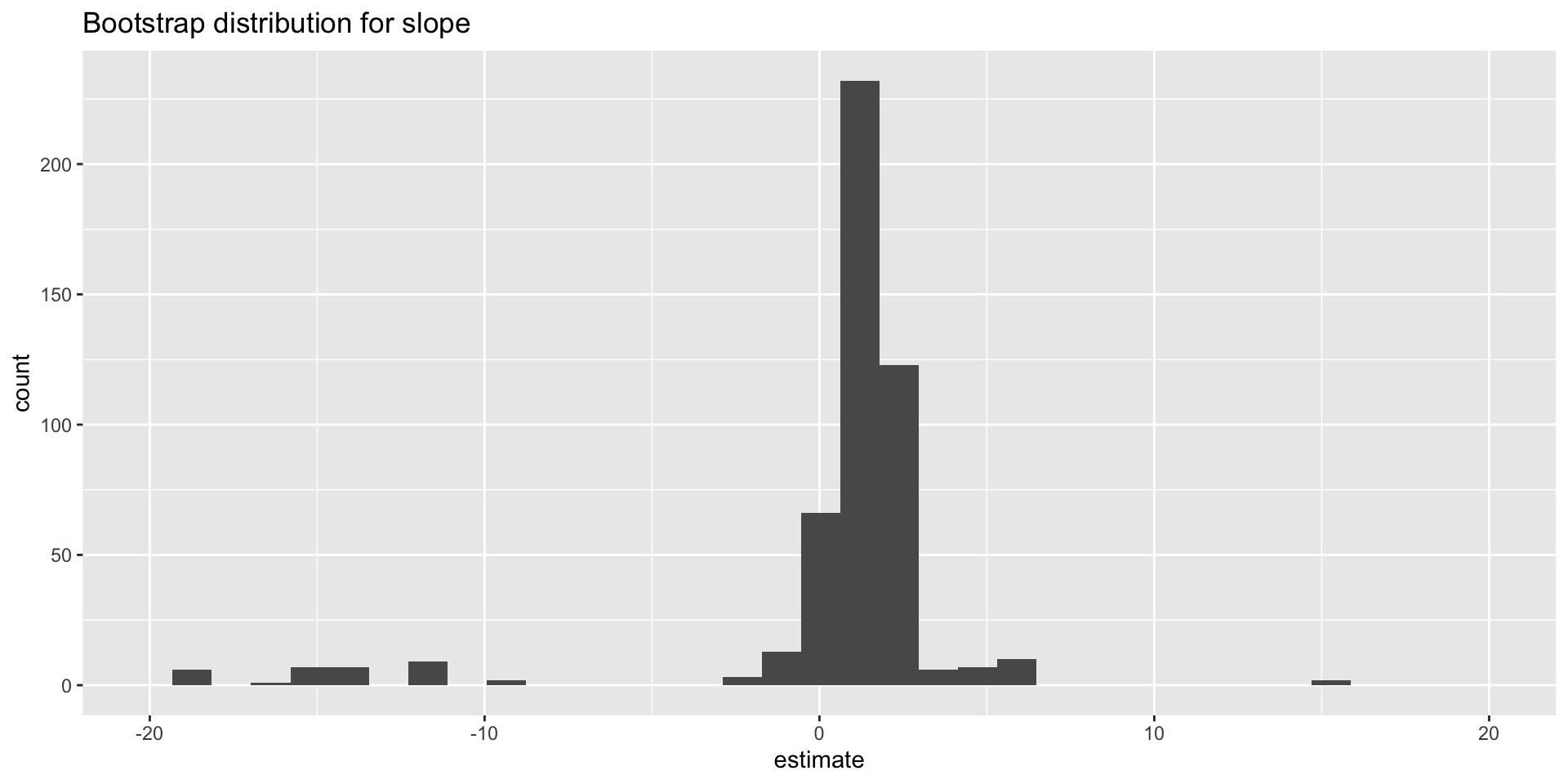
Model fit with five observations

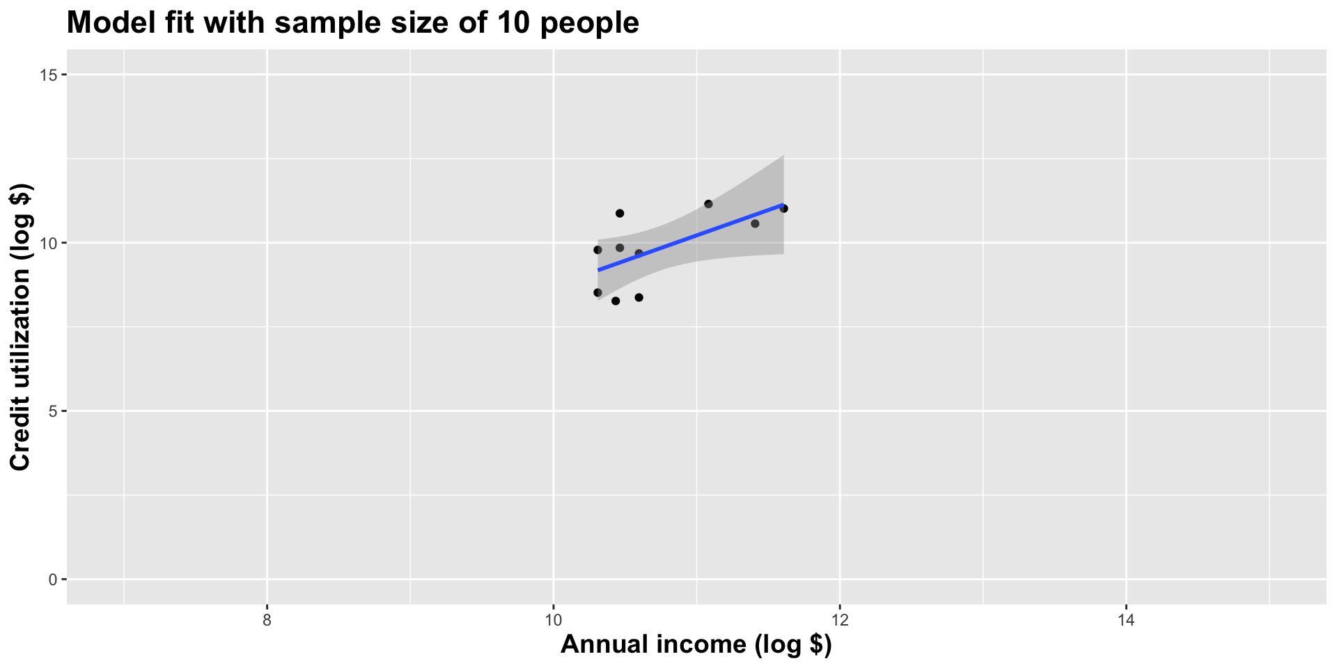
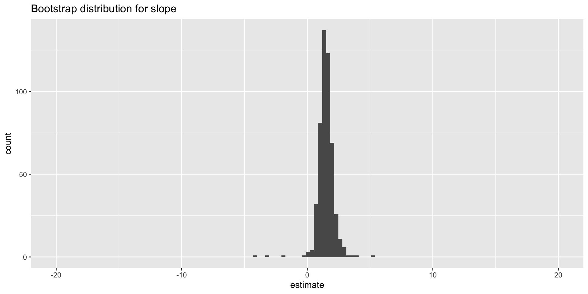
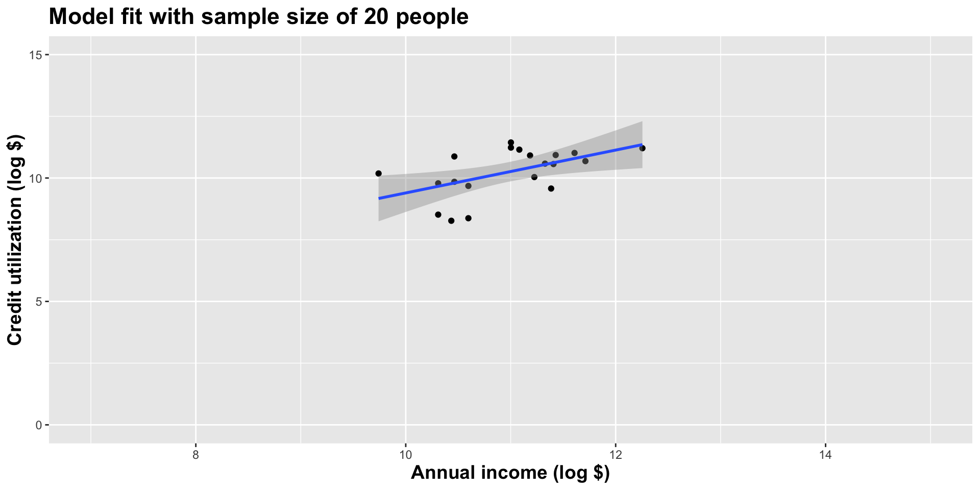
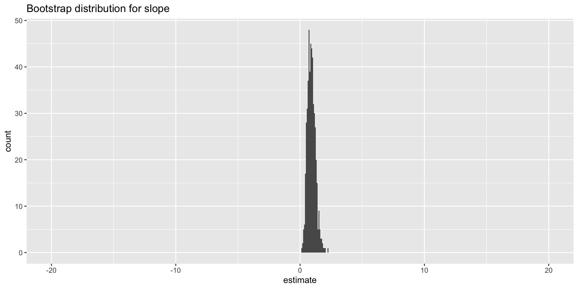
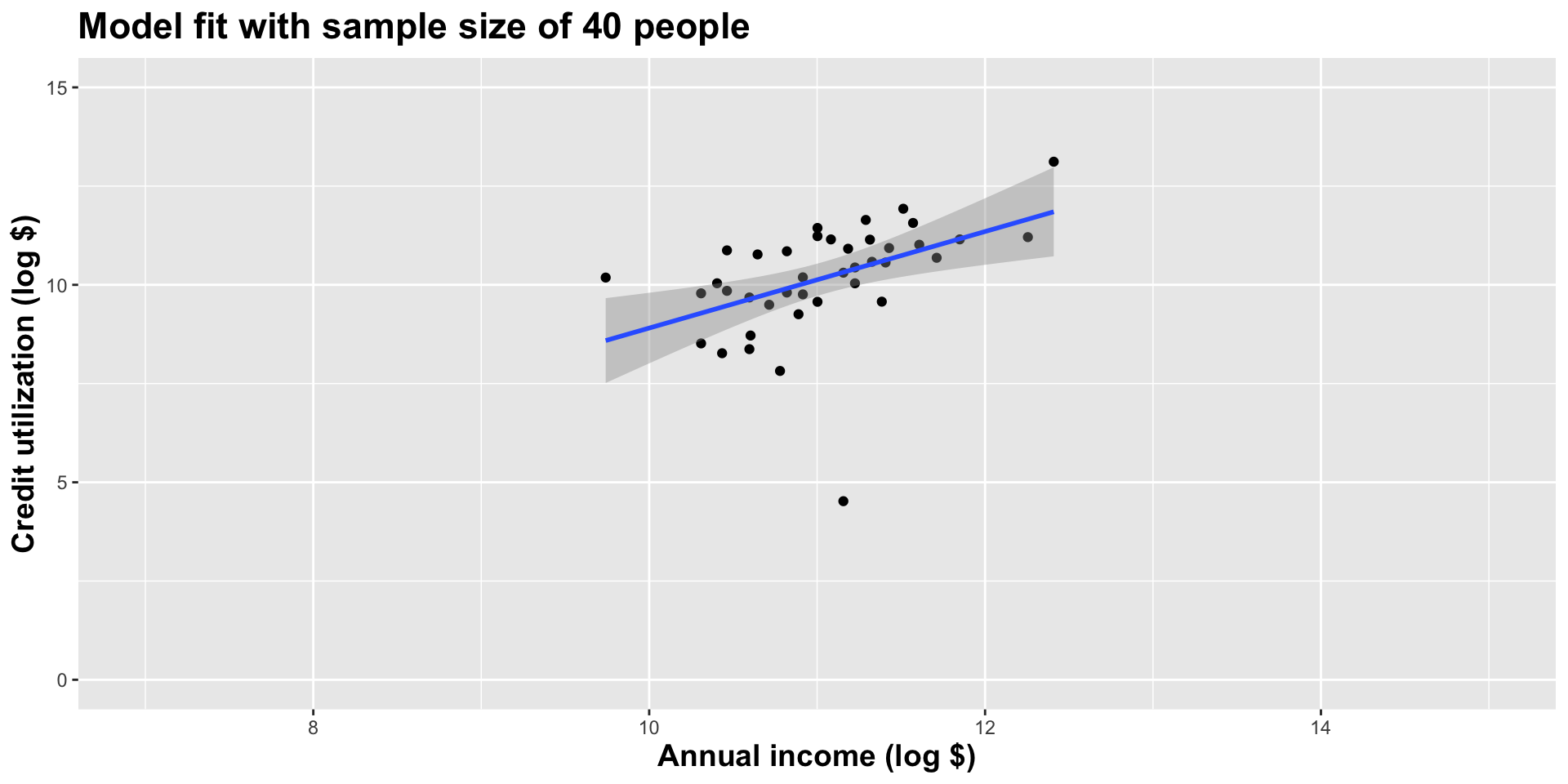
Double the sample size

Double the sample size again

Double the sample size again

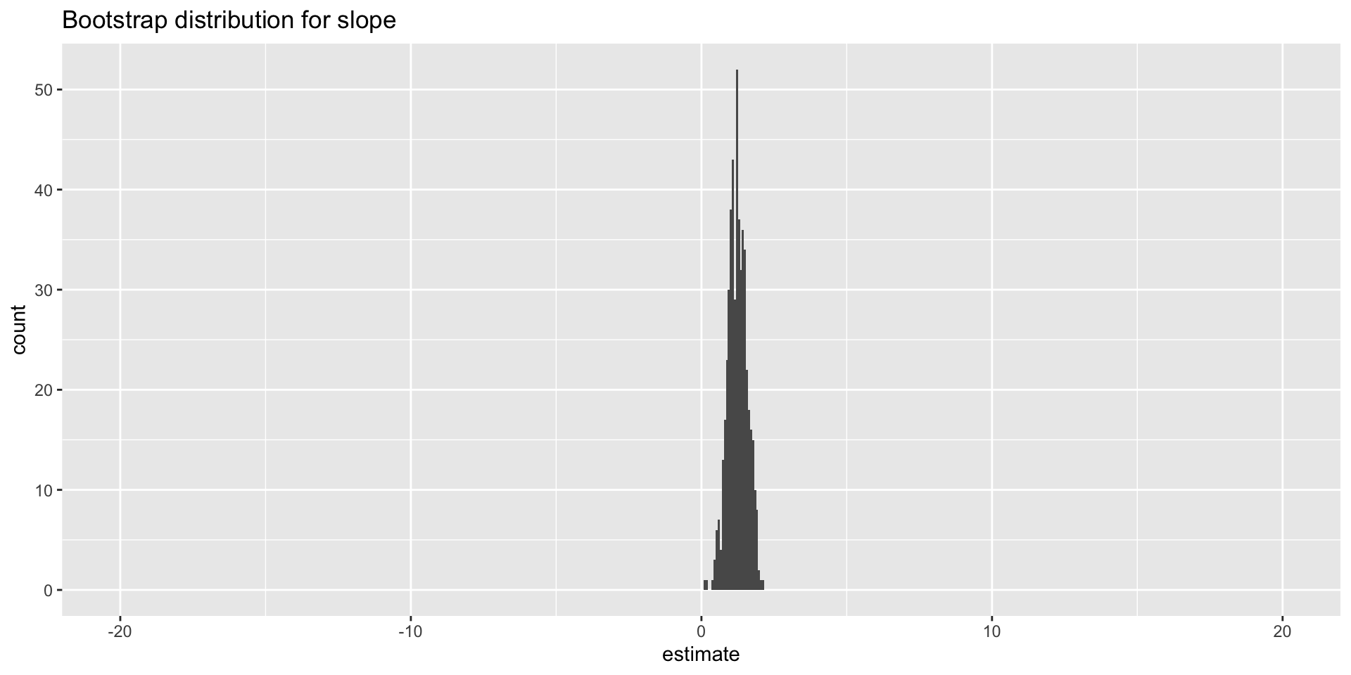
Double the sample size again

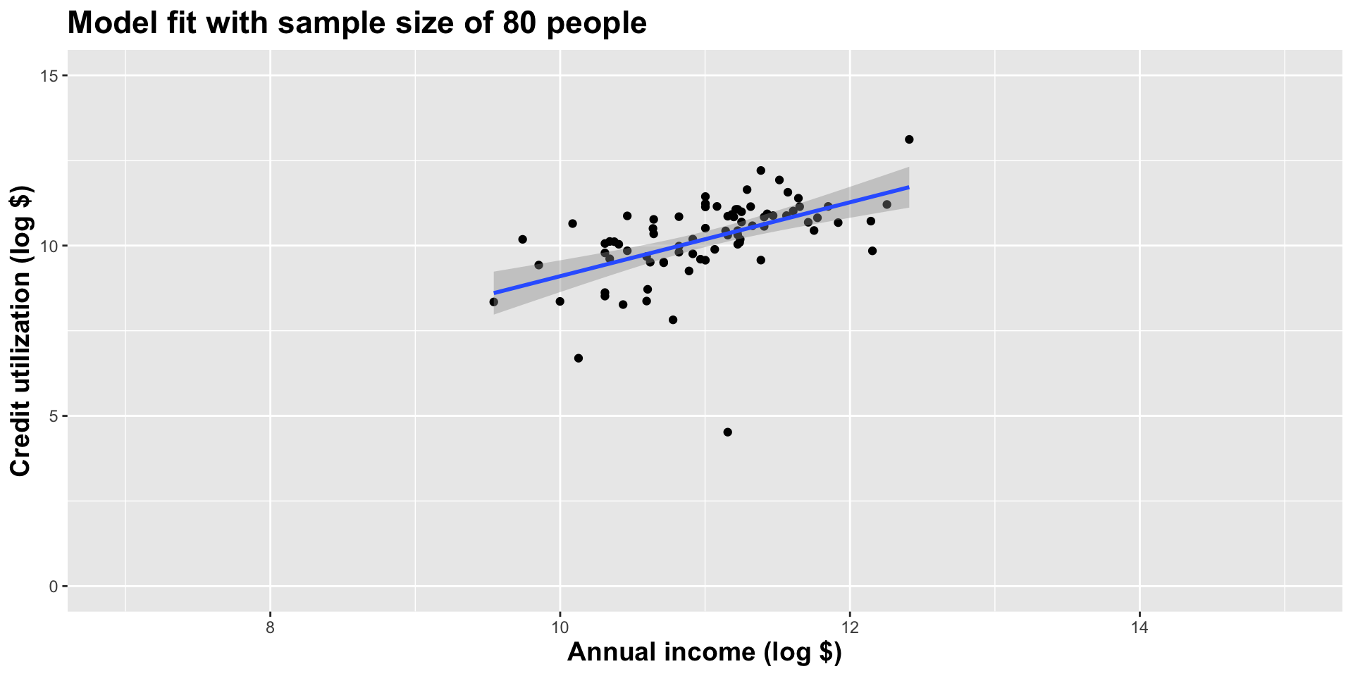
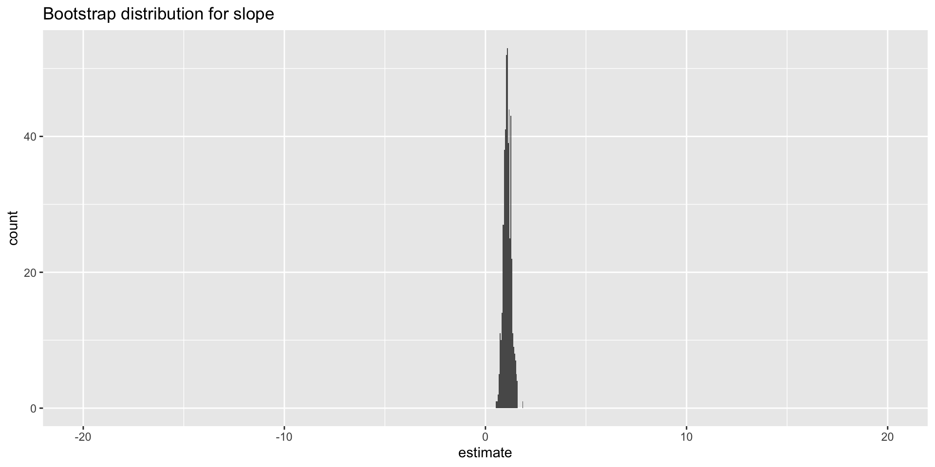
Double the sample size again

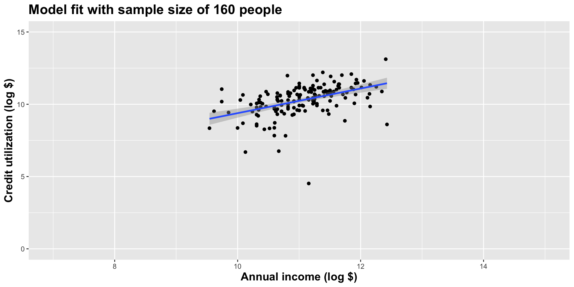
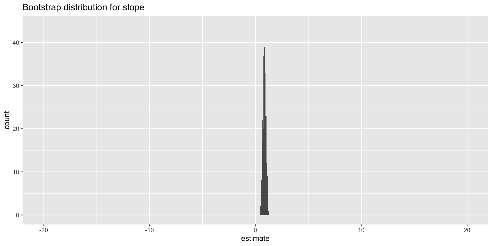
Double the sample size again

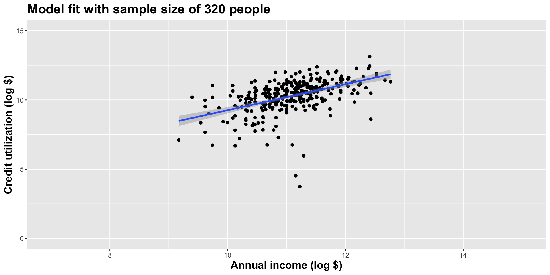
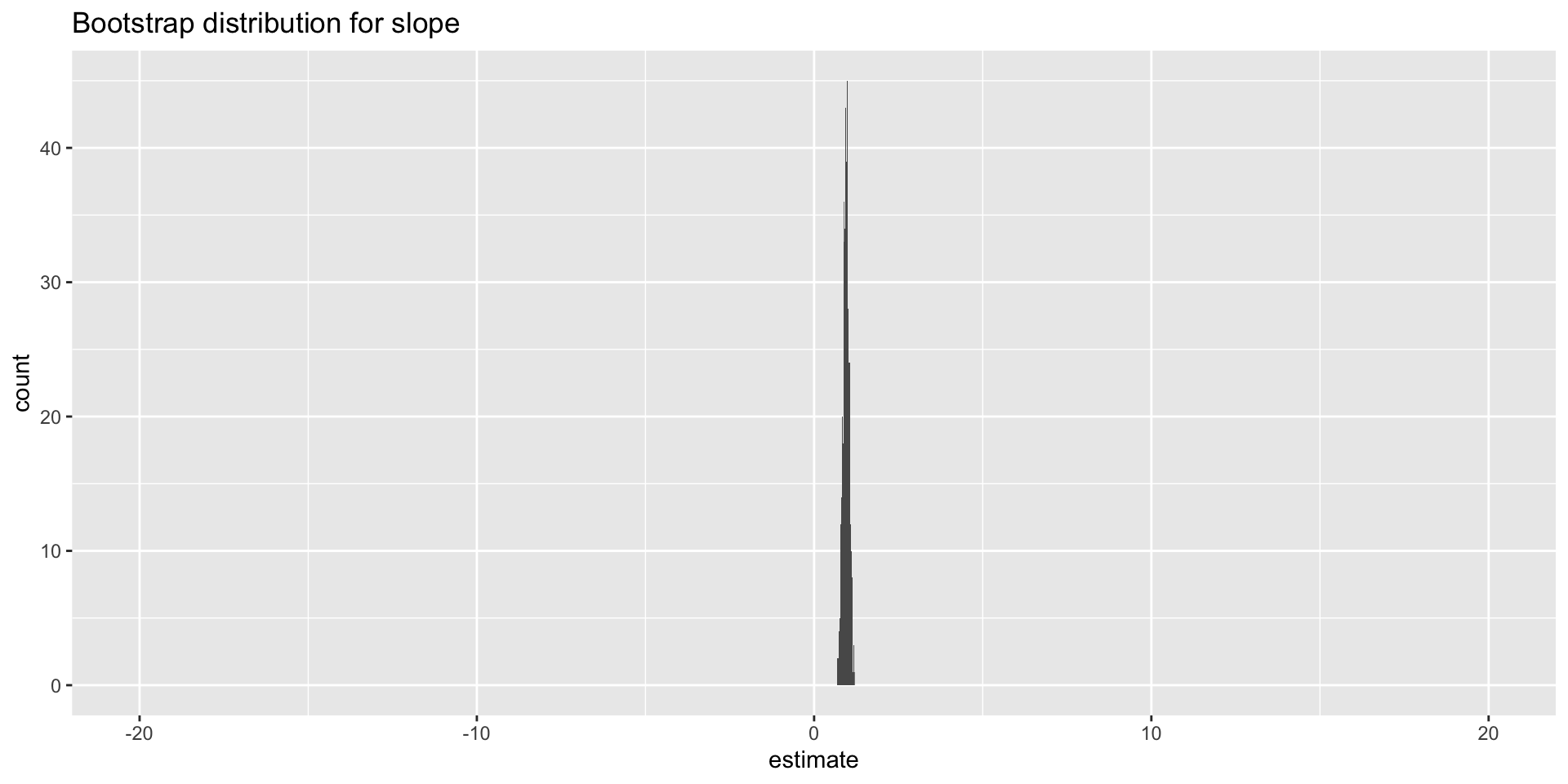
Double the sample size again

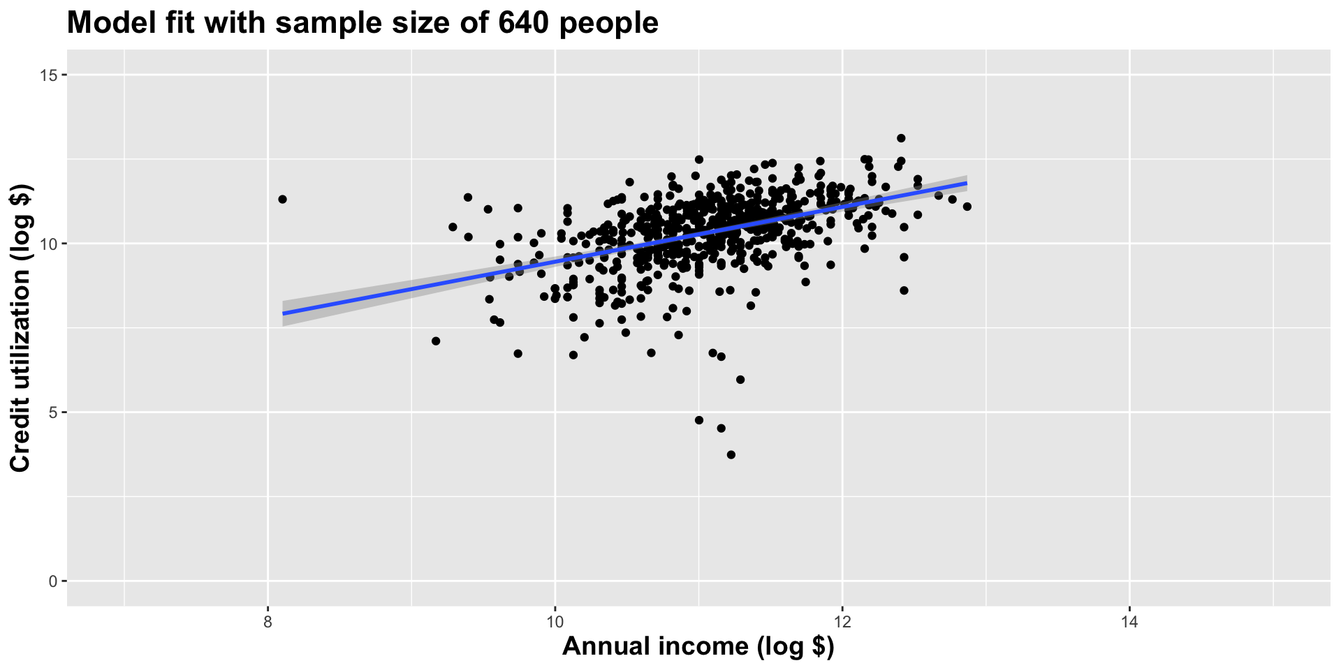
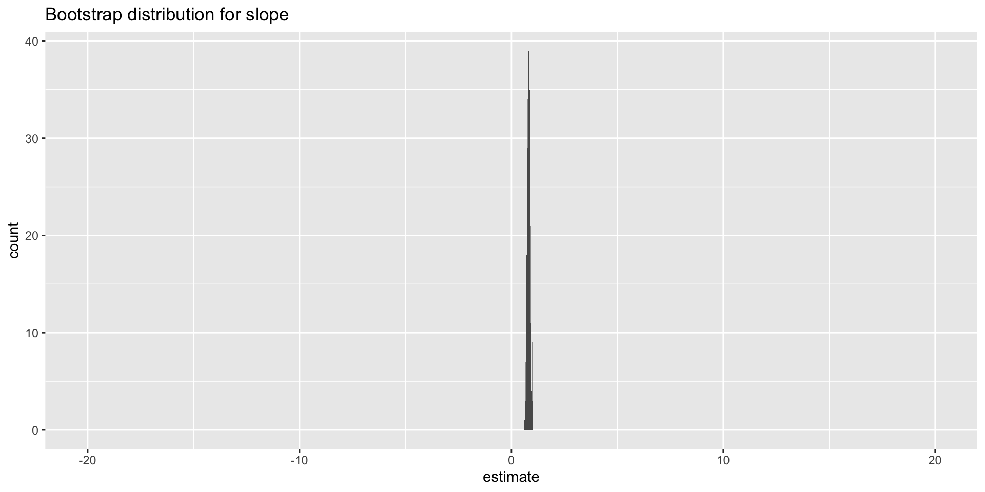
Double the sample size again

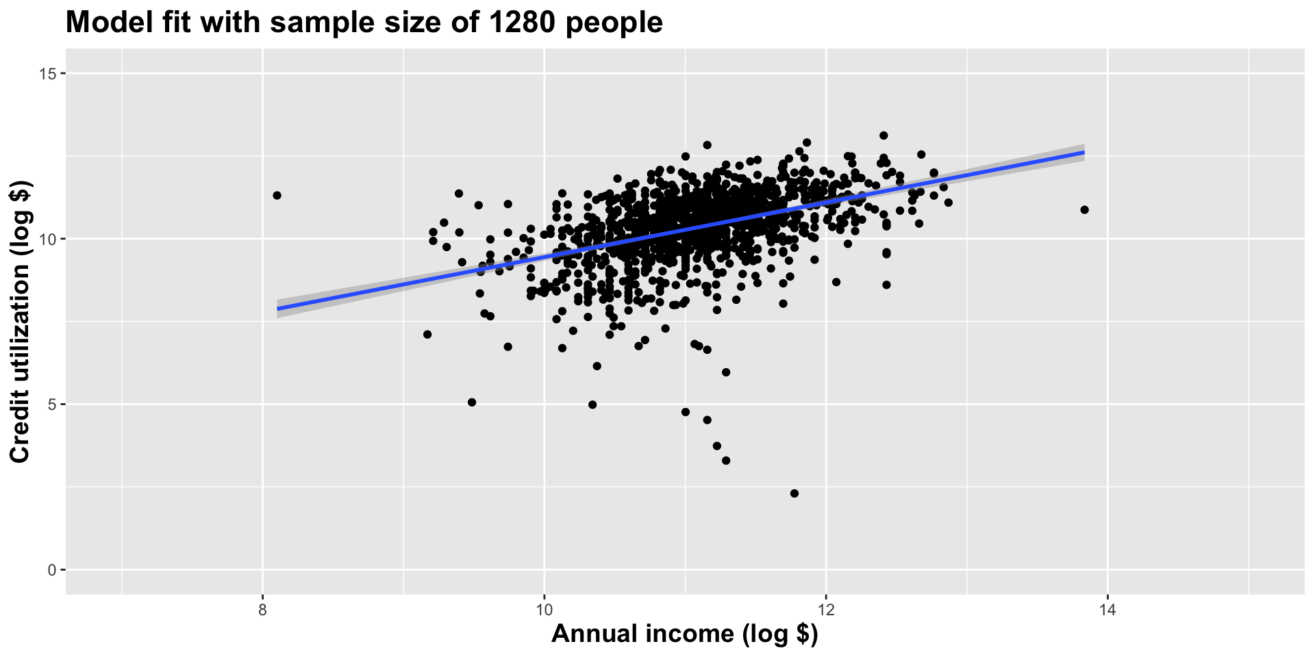
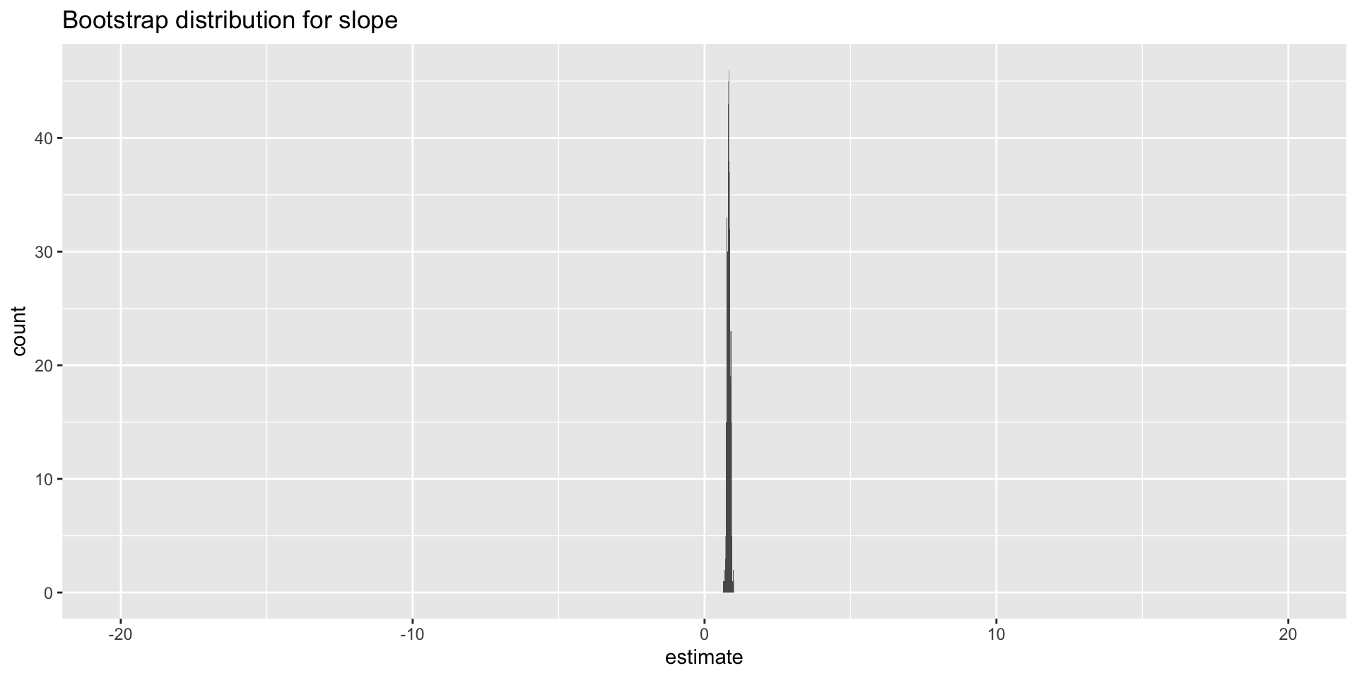
Double the sample size yet again

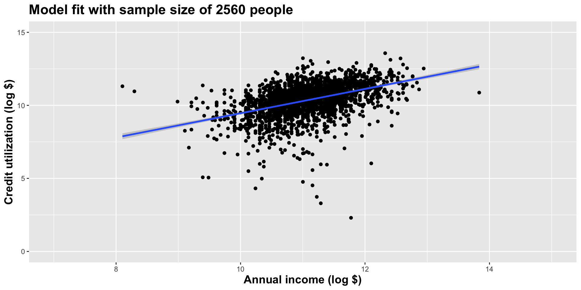
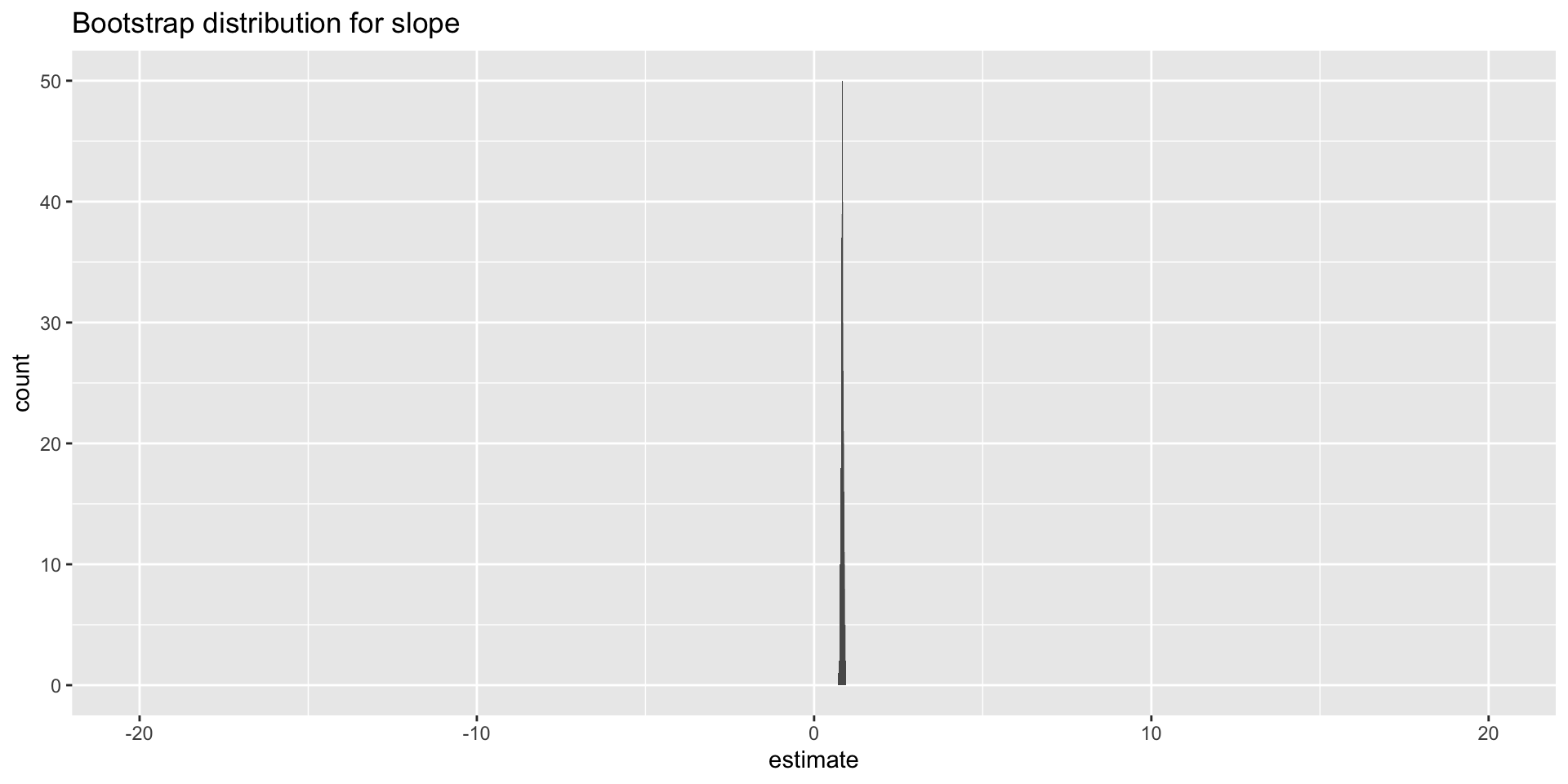
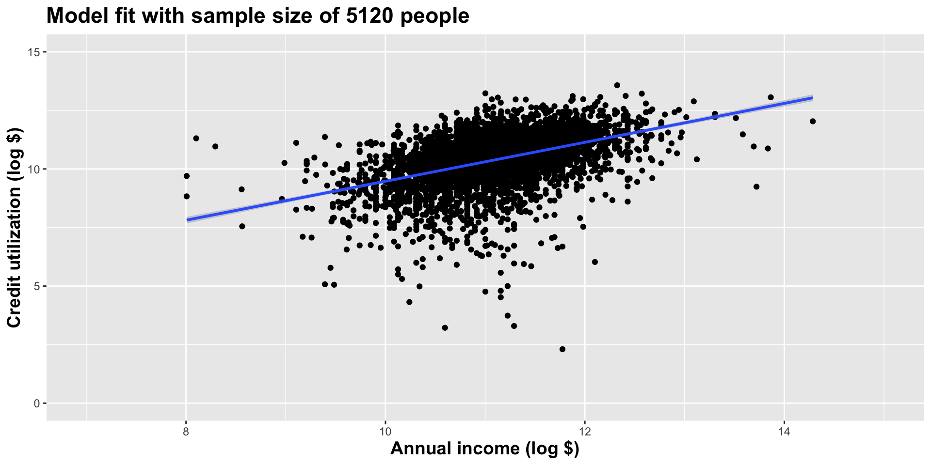
Double the sample size one more time

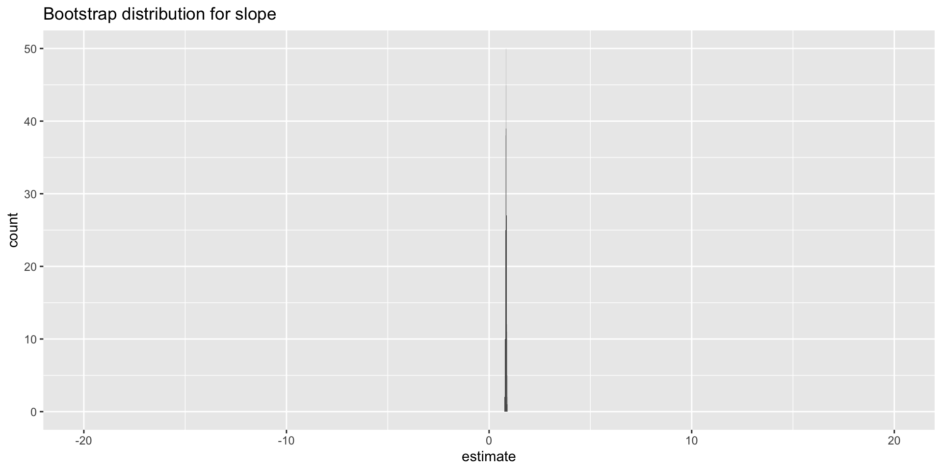
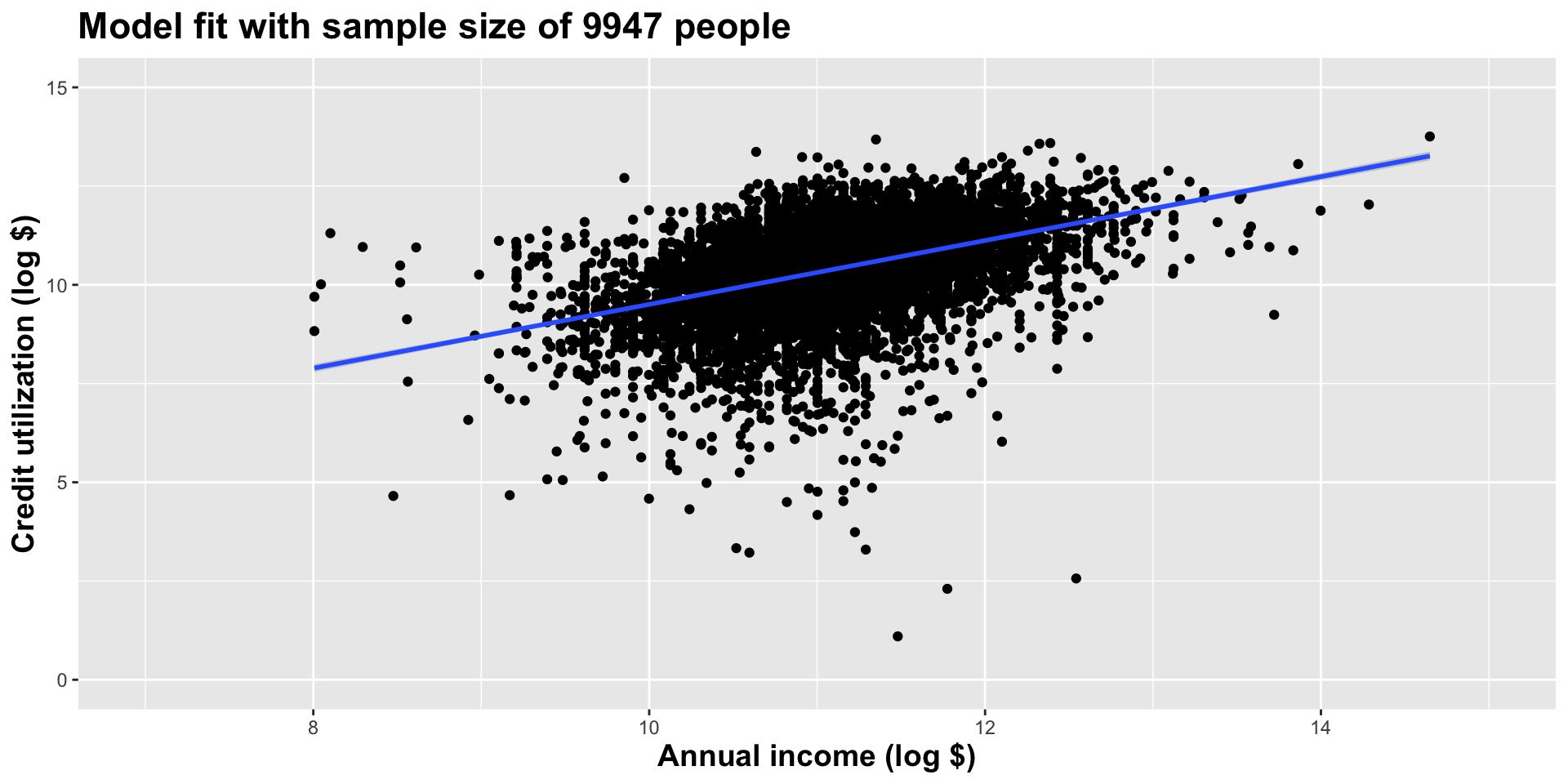
Use all the data we have

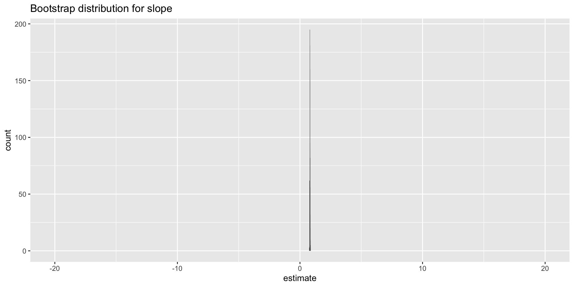
Let’s zoom in on that last distribution

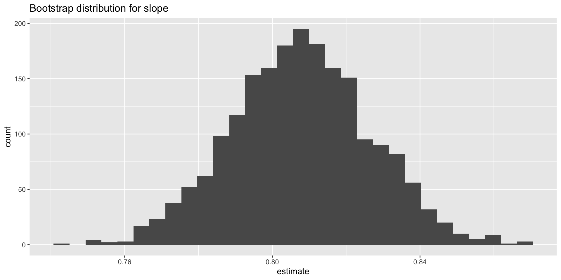
Two observations

Sampling distribution gets more concentrated in one spot;
The shape resembles a bell curve more and more.

These are not accidents!

The central limit theorem

Theorem

As your sample size gets bigger and bigger, the sampling distribution of many statistics (OLS slope, sample mean, sample proportion, etc) will look more and more like a bell curve that is concentrating around the true value you are trying to estimate.

For the proof, take STA 240 and beyond!

Upshot

Instead of using simulation and histograms to approximate sampling and null distributions, we can use the bell curve;
We can use mathematical facts about the bell curve to compute confidence intervals and p-values;
Before computers, this was the only game in town. Nowadays, you can just simulate. The results will probably be similar, especially when the sample size is large;
Nevertheless, old school normal approximations are still used often, so let’s talk about them.

The normal distribution (AKA the bell curve)

The bell curve

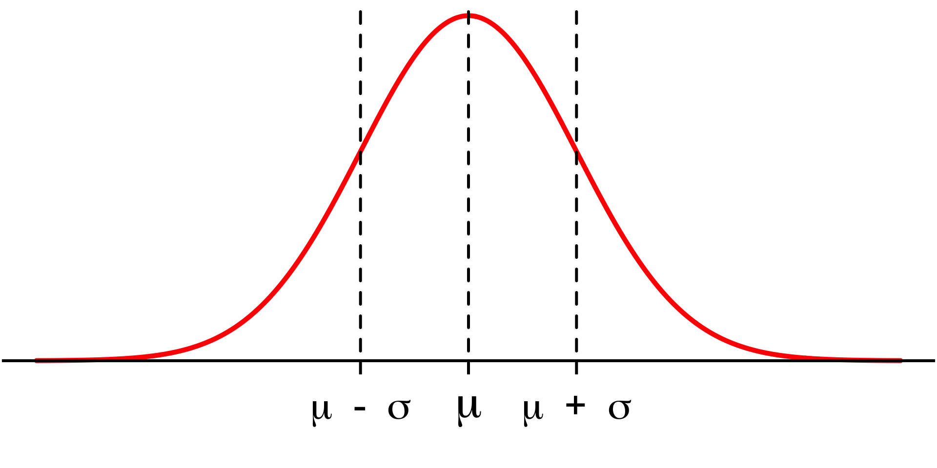
Notation: $N(\mu,\,\sigma)$

$\mu$ (“mu”) is the mean. Controls center;
$\sigma$ (“sigma”) is the standard deviation. Controls spread.

The bell curve

#| '!! shinylive warning !!': |
#|   shinylive does not work in self-contained HTML documents.
#|   Please set `embed-resources: false` in your metadata.
#| standalone: true
#| viewerHeight: 500

library(shiny)

ui <- fluidPage(
  titlePanel("The normal distribution"),
  sidebarLayout(
    sidebarPanel(
      sliderInput(
        inputId = "mu",
        label = "Mean (μ)",
        min = -5,
        max = 5,
        value = 0,
        step = 0.1
      ),
    
      sliderInput(
        inputId = "sigma",
        label = "Standard deviation (σ)",
        min = 0.5,
        max = 3,
        value = 1,
        step = 0.1
      )
    ),
    
    mainPanel(
      plotOutput("density_plot")
    )
  )
)

server <- function(input, output) {

  output$density_plot <- renderPlot({

    x <- seq(-10, 10, length.out = 1000)
    y <- dnorm(x, mean = input$mu, sd = input$sigma)

    plot(
      x, y,
      type = "l",
      col = "steelblue",
      lwd = 3,
      xlim = c(-10, 10),
      ylim = c(0, 0.85),
      xlab = "x",
      ylab = "Density",
      main = paste0("N(", input$mu, ", ", input$sigma, ")")
    )

    polygon(
      c(x, rev(x)),
      c(y, rep(0, length(y))),
      col = adjustcolor("steelblue", alpha.f = 0.2),
      border = NA
    )

    #abline(v = input$mu, col = "firebrick", lty = 2, lwd = 2)

  })

}

shinyApp(ui, server)

The 68–95–99.7 rule

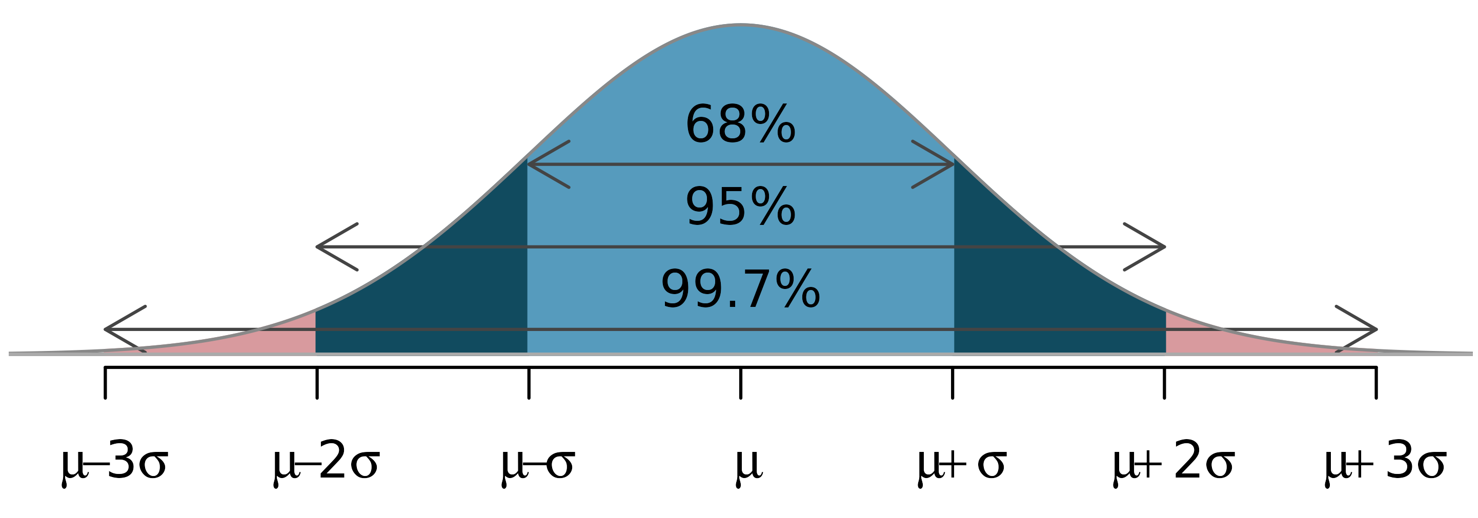
Let’s practice!

(in the container)

Inference with normal approximations (instead of simulation)

The main idea

The central limit theorem (CLT) says that if our sample size ($n$) is “large enough,” then our estimate of the slope ($b_1$) varies across datasets according to

\[ N(\text{mean} = \beta_1,\,\text{sd}=\text{SE}) \]

$\beta_1$ is the “true value” of the slope. Gosh we wish we knew it. It’s the ideal but unknown reference point that our estimates are wiggling around;
“SE” stands for “standard error.” It’s just special vocabulary for the standard deviation of a sampling distribution. We’ll worry about how it’s calculated later.

The standard error

\[ N(\text{mean} = \beta_1,\,\text{sd}=\text{SE}) \]

The standard error measures the spread of the sampling distribution, which communicates uncertainty about the estimate. SE higher bad; SE lower good.

The value of the SE is influenced by two factors:

the variability of the data: the more “all over the place” your data are, the less reliable the estimates, so SE goes up;
sample size: the more (less) data you have, the lower (higher) the SE.

So, the SE is a tug-of-war between the noisiness of the data and how much of it you have.

Approximation

\[ N(\text{mean} = \beta_1,\,\text{sd}=\text{SE}) \]

Using this is just as much an approximation as simulation + histogram;
The bell curve only works for $n$ “large enough;”
Both $\beta_1$ and SE are unknown. They need to be approximated from the data;
- For $\beta_1$, we naturally use $b_1$;
- Don’t worry about SE just yet. For now, be content that the computer can estimate it…

The standard error

It’s been staring us in the face the entire time:

linear_reg() |>
  fit(mpg ~ wt, data = mtcars) |>
  tidy()

# A tibble: 2 × 5
  term        estimate std.error statistic  p.value
  <chr>          <dbl>     <dbl>     <dbl>    <dbl>
1 (Intercept)    37.3      1.88      19.9  8.24e-19
2 wt             -5.34     0.559     -9.56 1.29e-10

So how do we use it for interval estimation and hypothesis testing?

Inference with the normal distribution

The story so far

Our statistical problem

Grand summary from last time

The main ideas

We must approximate!

Recall this example

Model fit with three observations

Model fit with five observations

Double the sample size

Double the sample size again

Double the sample size again

Double the sample size again

Double the sample size again

Double the sample size again

Double the sample size again

Double the sample size again

Double the sample size yet again

Double the sample size one more time

Use all the data we have

Let’s zoom in on that last distribution

Two observations

The central limit theorem

Upshot

The normal distribution (AKA the bell curve)

The bell curve

The bell curve

The 68–95–99.7 rule

Let’s practice!

Inference with normal approximations (instead of simulation)

The main idea

The standard error

Approximation

The standard error

Back to the containers!