Lecture 9
Duke University
STA 101 Fall 2026
2026-09-29
We have been studying regression:
What combinations of data types have we seen?
What did the picture look like?
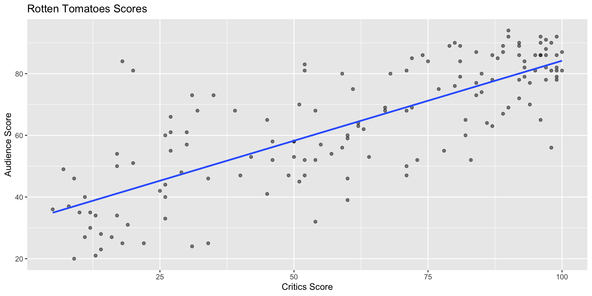
Numerical response and one numerical predictor:
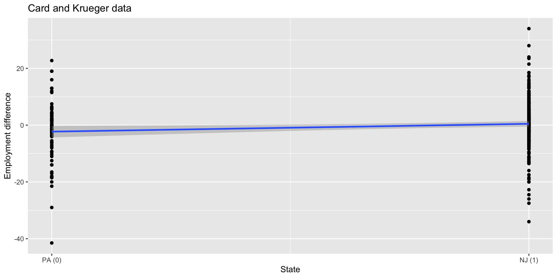
Numerical response and one categorical predictor (two levels):
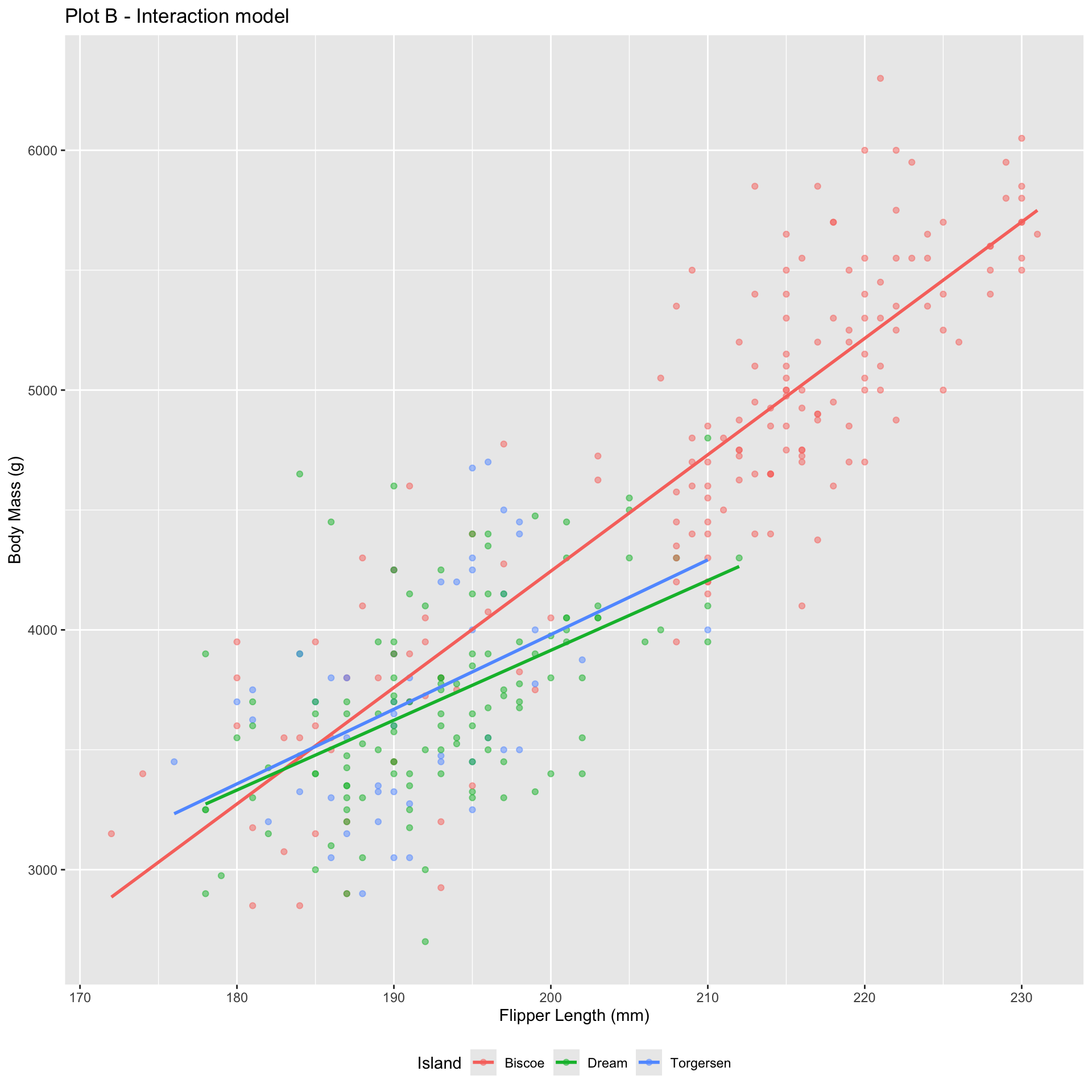
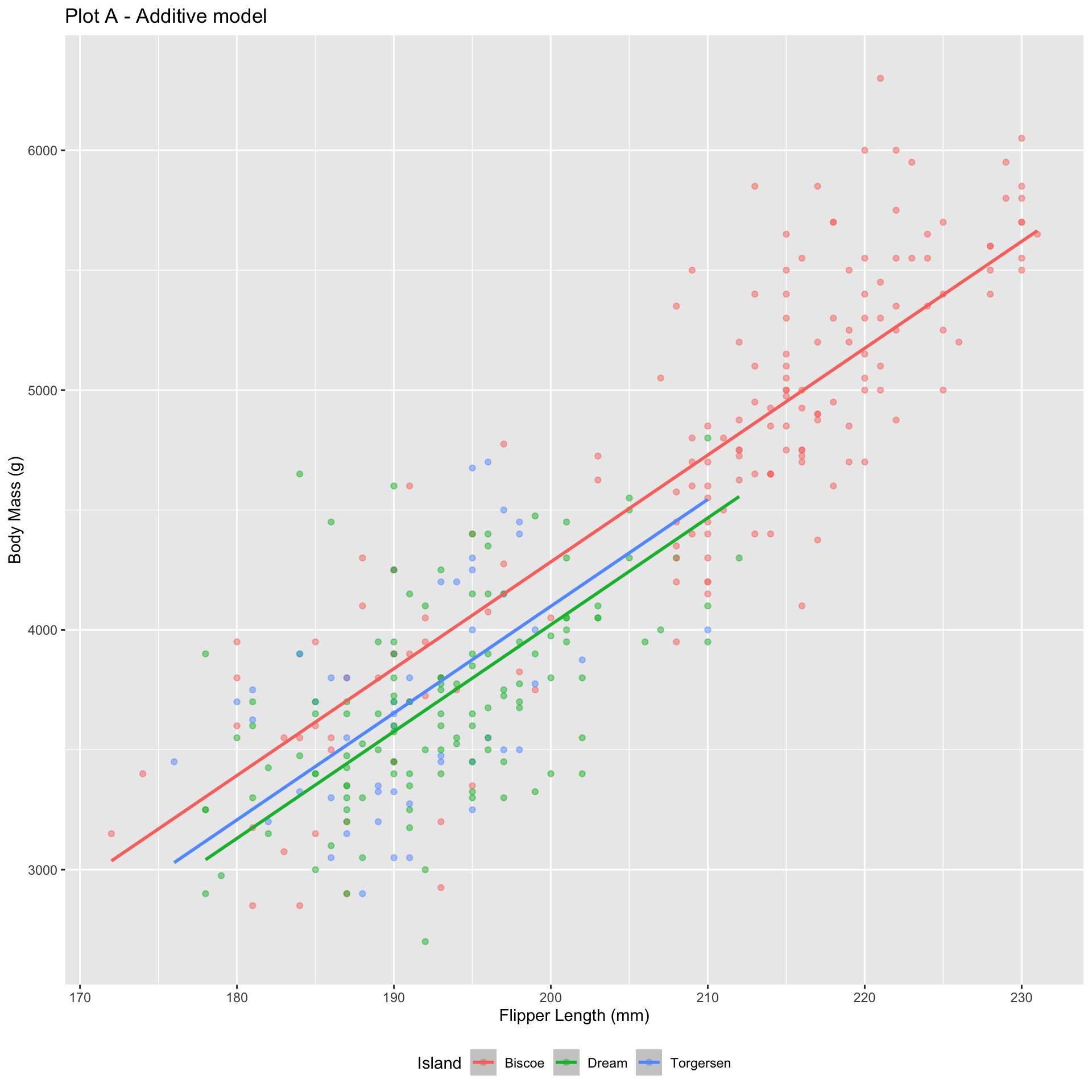
Numerical response; numerical and categorical predictors:

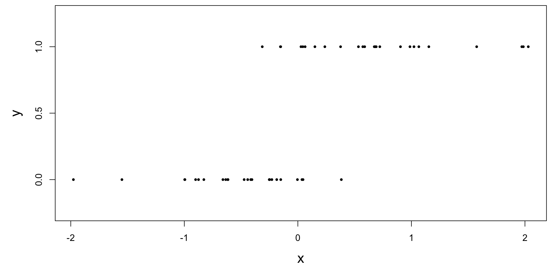
\[ y = \begin{cases} 1 & &&\text{eg. Yes, Win, True, Heads, Success}\\ 0 & &&\text{eg. No, Lose, False, Tails, Failure}. \end{cases} \]
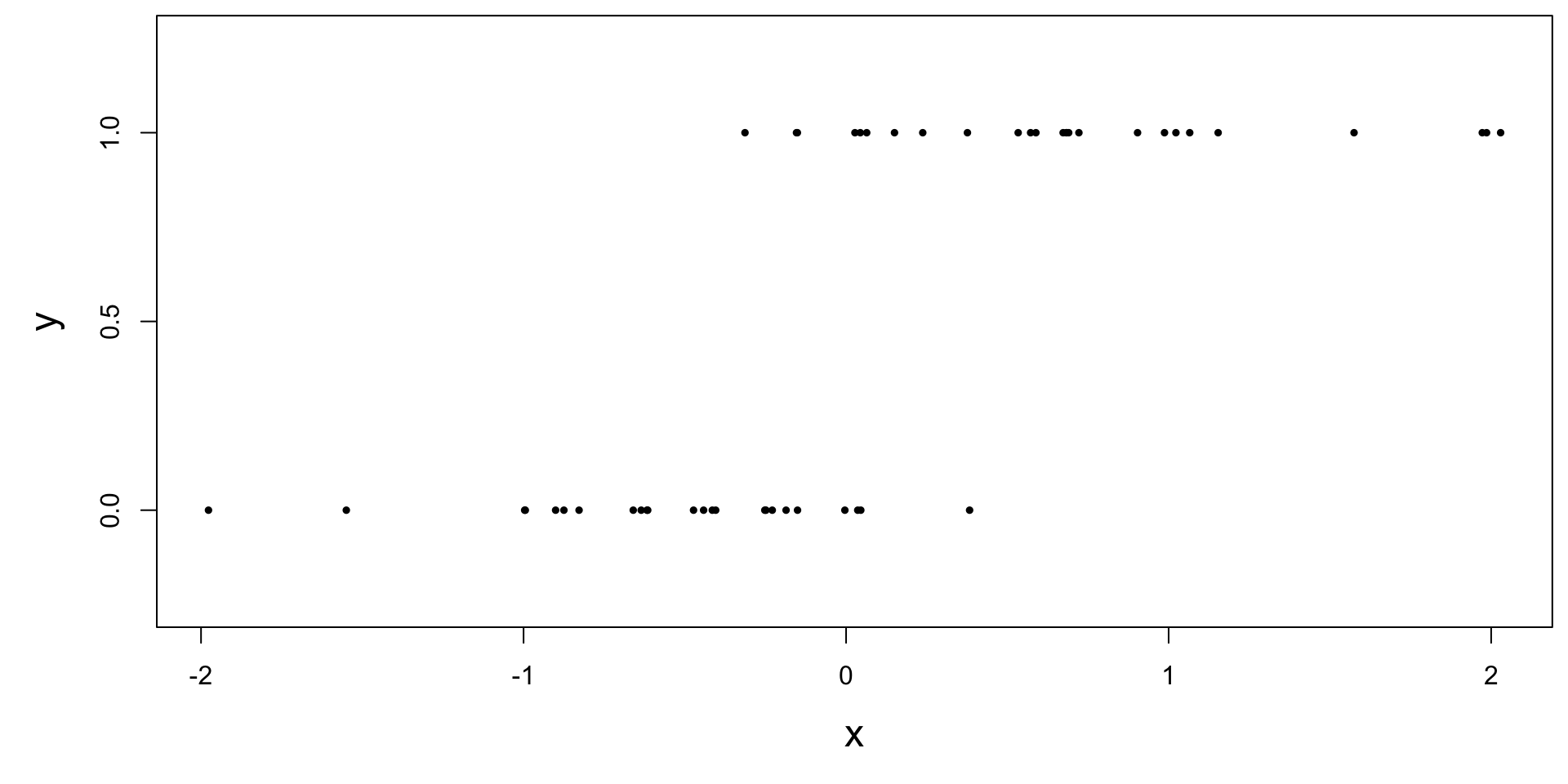
If we can model the relationship between predictors (\(x\)) and a binary response (\(y\)), we can use the model to do a special kind of prediction called classification.
\[ \mathbf{x}: \text{word and character counts in an e-mail.} \]

\[ y = \begin{cases} 1 & \text{it's spam}\\ 0 & \text{it's legit} \end{cases} \]
\[ \mathbf{x}: \text{features in a medical image.} \]
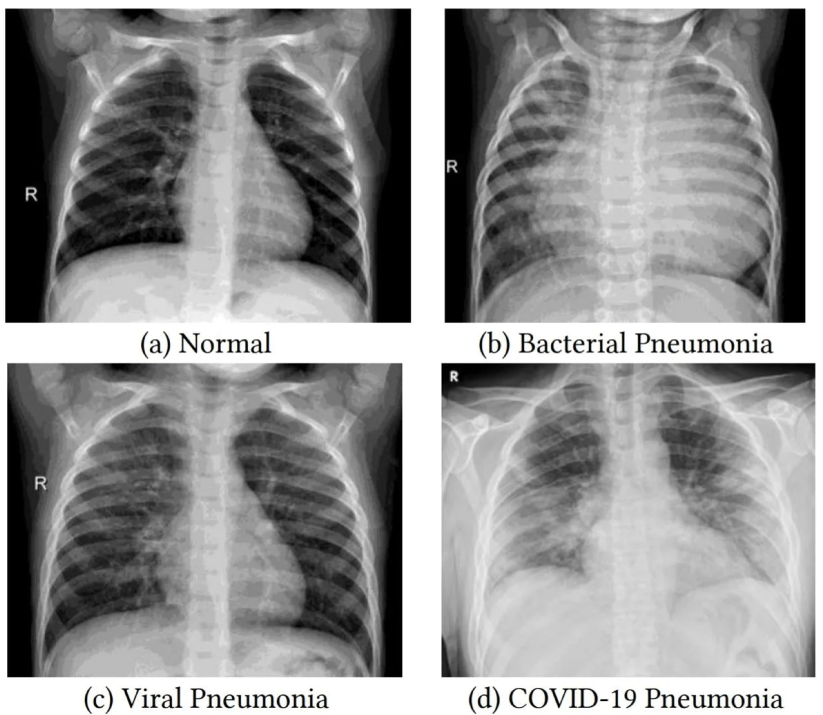
\[ y = \begin{cases} 1 & \text{it's pneumonia}\\ 0 & \text{it's healthy} \end{cases} \]
\[ \mathbf{x}: \text{financial and demographic info about a loan applicant.} \]
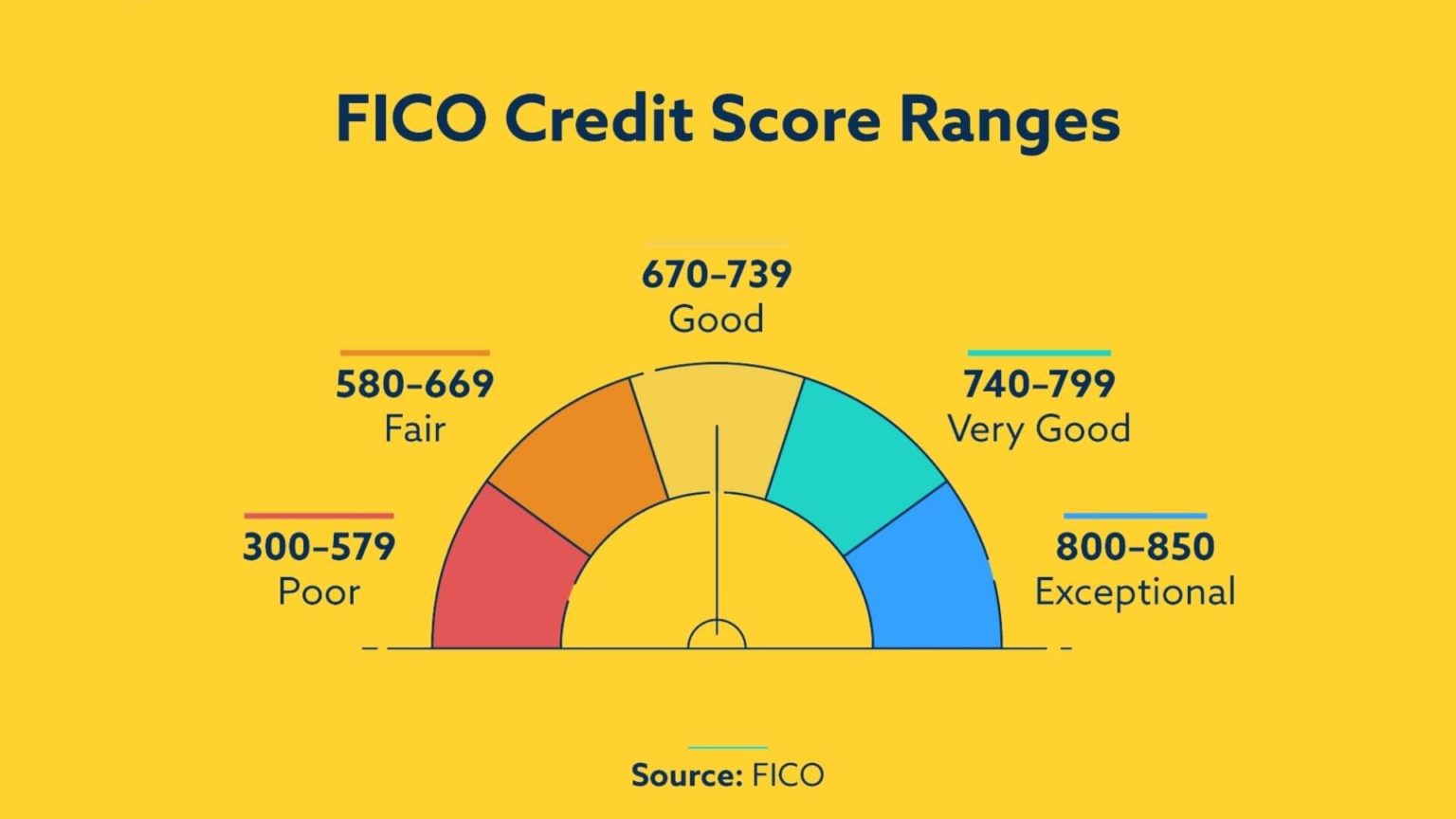
\[ y = \begin{cases} 1 & \text{applicant is at risk of defaulting on loan}\\ 0 & \text{applicant is safe} \end{cases} \]
\[ \mathbf{x}: \text{word counts (e.g., thou, love, heartbreak), stylistic features} \]

\[ y = \begin{cases} 1 & \text{Taylor Swift}\\ 0 & \text{William Shakespeare} \end{cases} \]
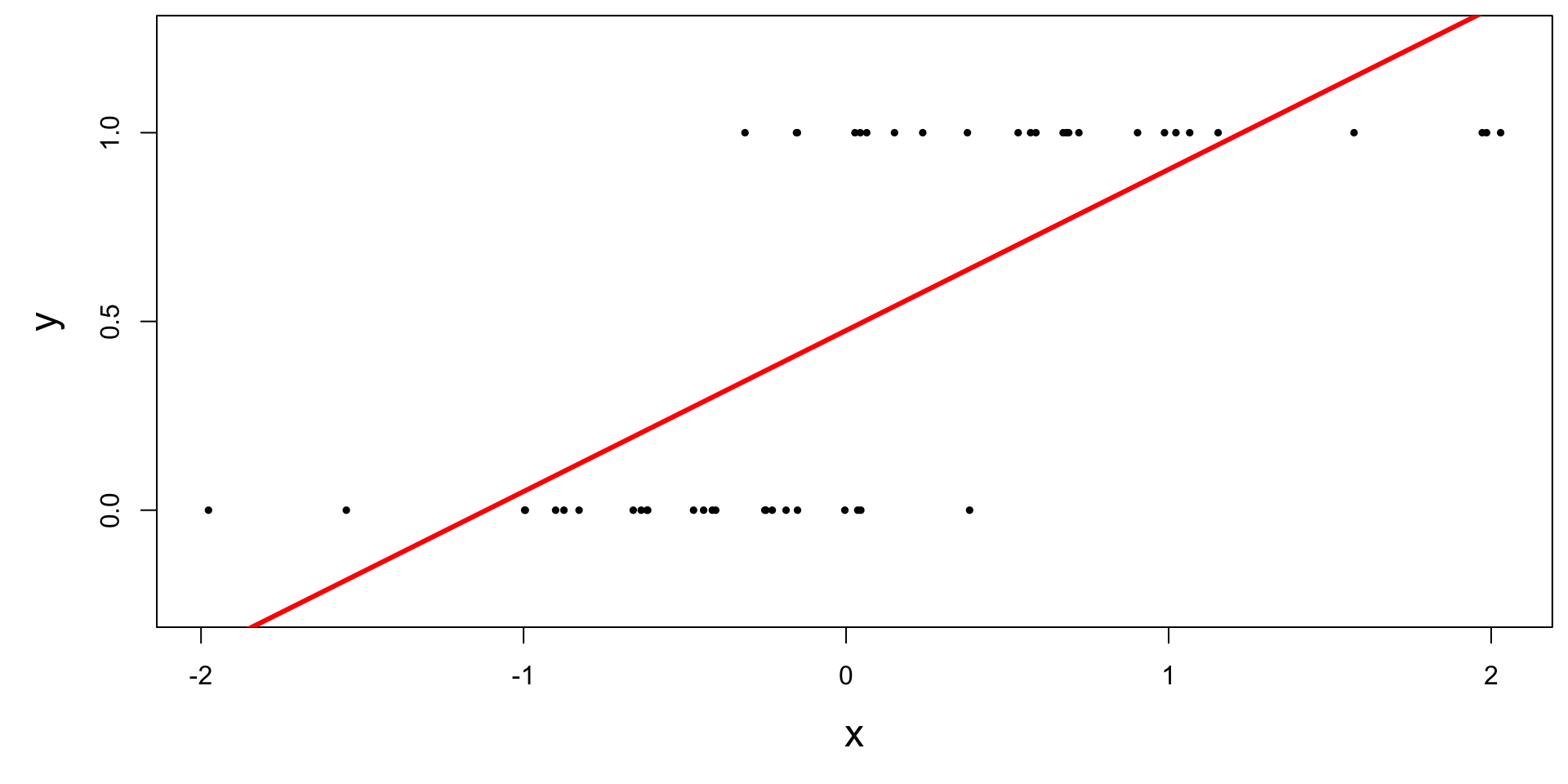
Possible, but silly.
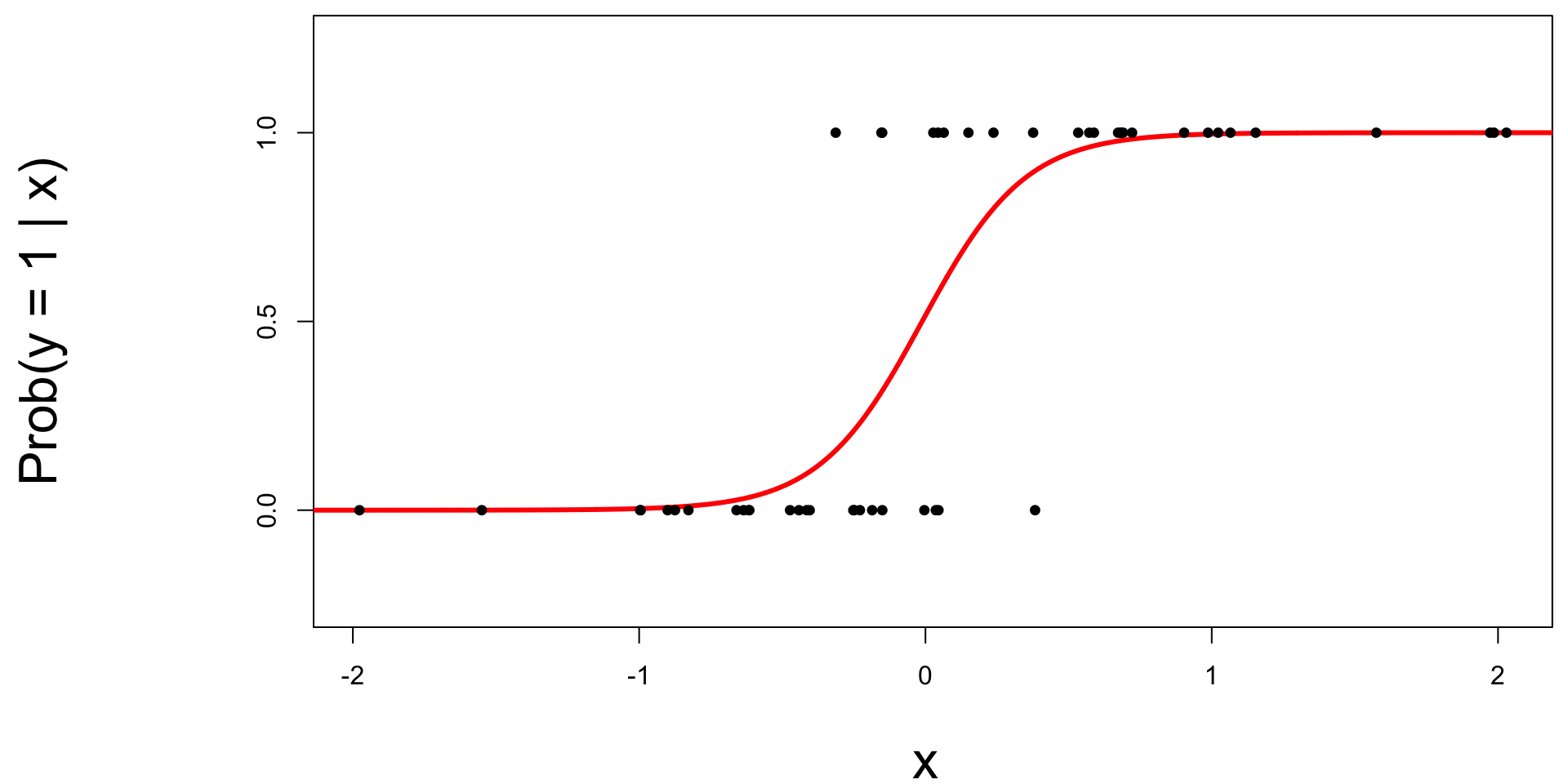
Instead of modeling \(y\) directly, we model the probability that \(y=1\):
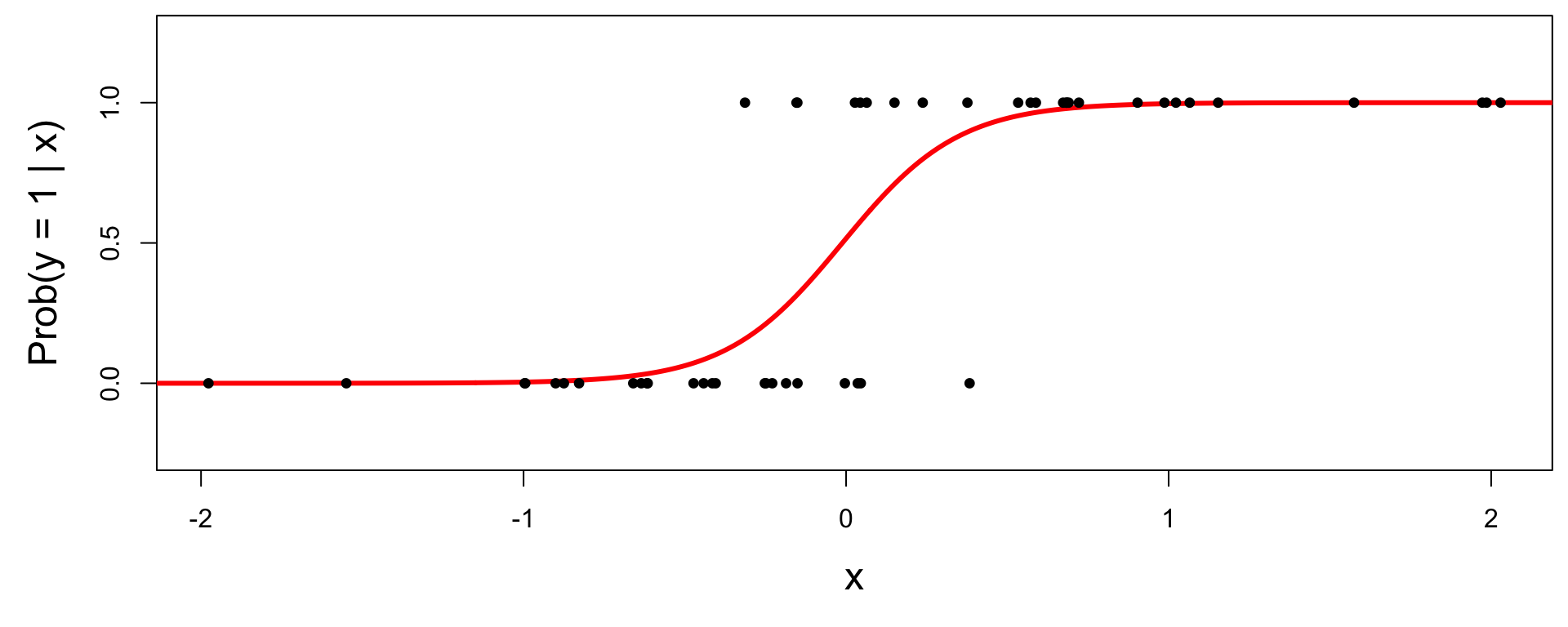
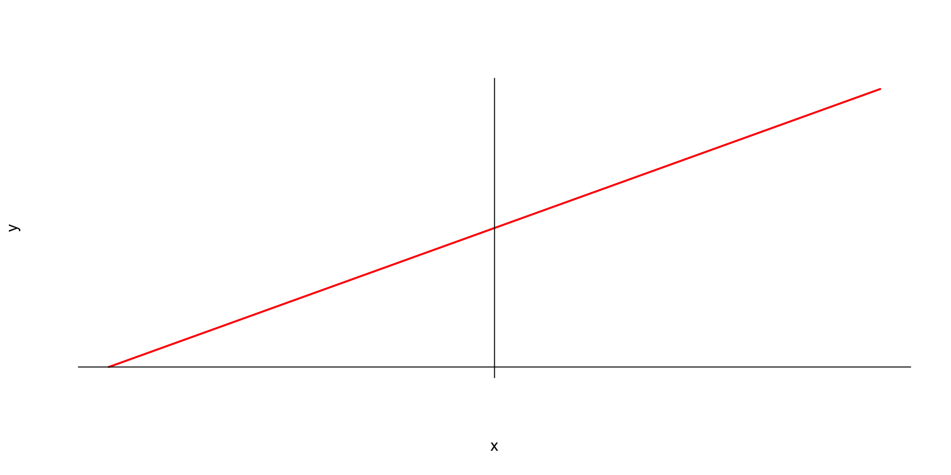
Recall regression with a numerical response:
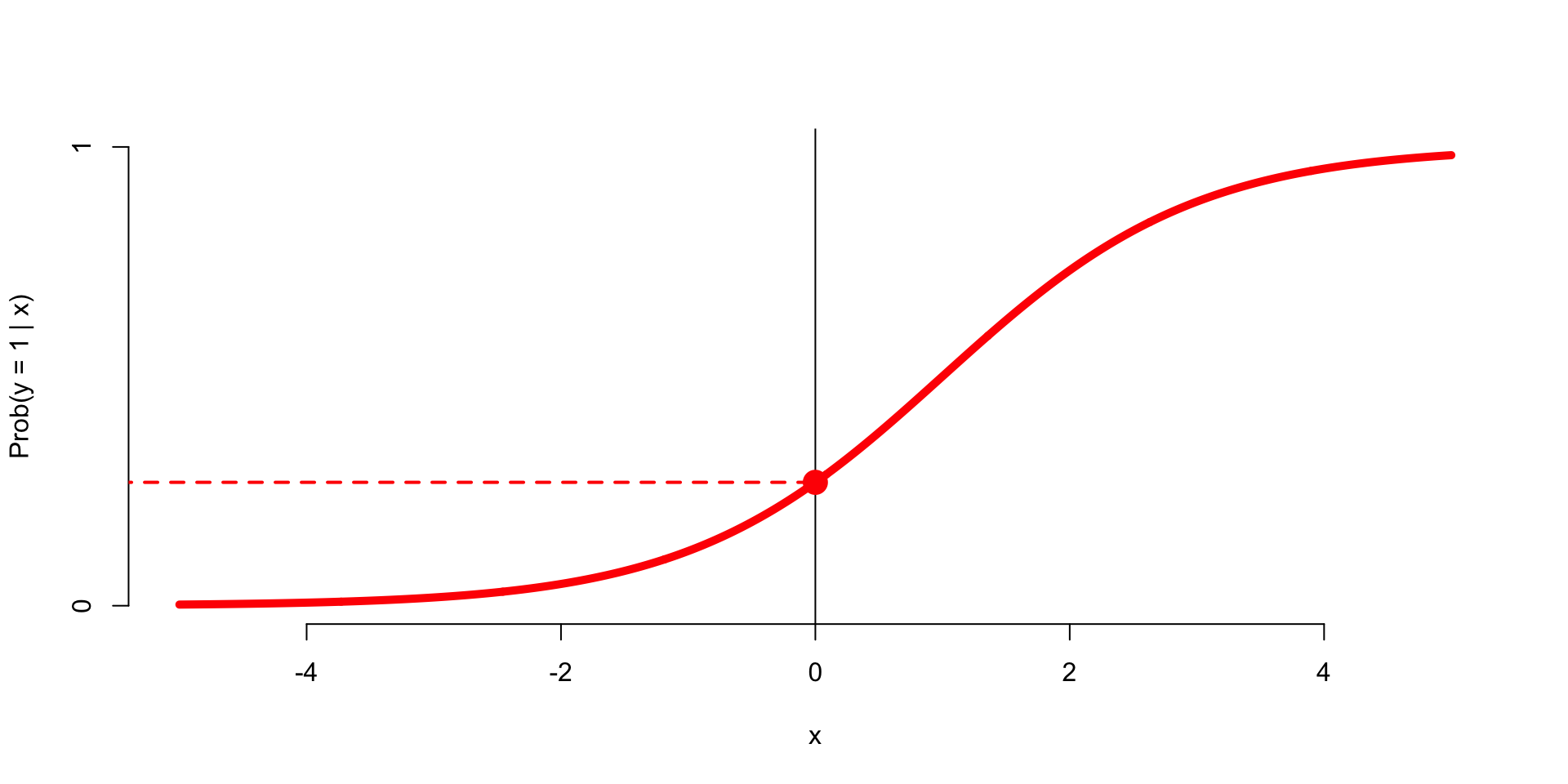
Similar when modeling a binary response:
\[ \text{Prob}(y = 1\mid x) = \frac{e^{\beta_0+\beta_1x}}{1+e^{\beta_0+\beta_1x}}. \]
If you set \(p = \text{Prob}(y = 1\mid x)\) and do some algebra, you get the simple linear model for the log-odds:
\[ \log\left(\frac{p}{1-p}\right) = \beta_0+\beta_1x. \]
This is called the logistic regression model.

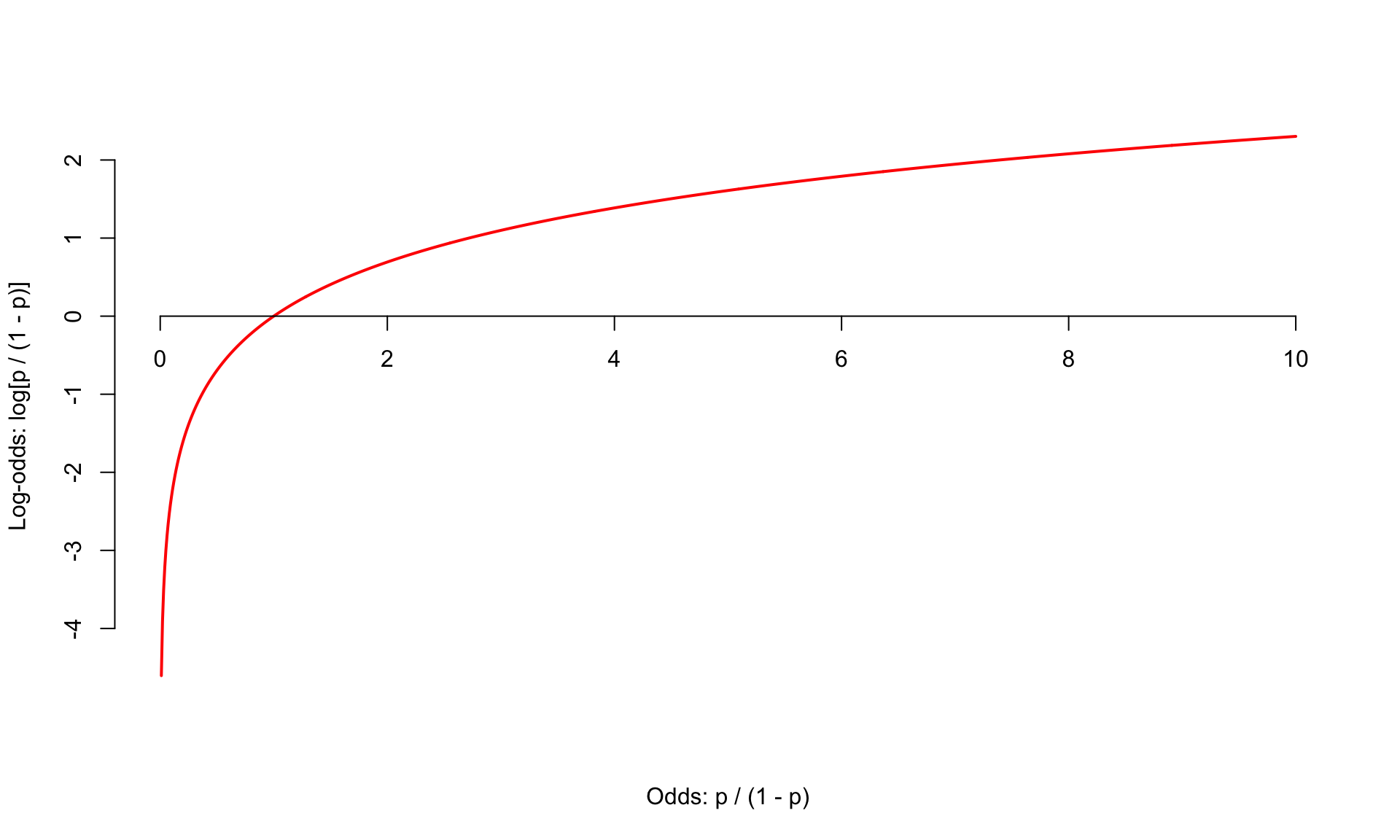
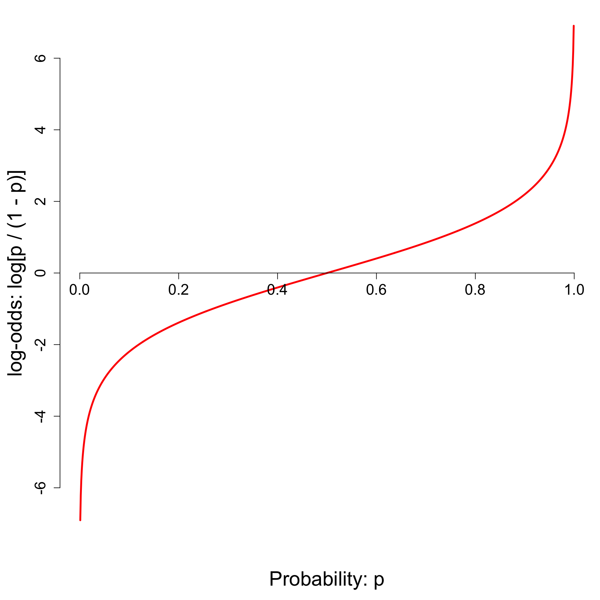
The log-odds transformation takes probabilities between 0 and 1 and streeetches them out to numbers between \(-\infty\) and \(\infty\), for which the linear model is appropriate.
\[ \log\left(\frac{p}{1-p}\right) = \beta_0+\beta_1x. \]
The logit function \(\log(p / (1-p))\) is an example of a link function that transforms the linear model to have an appropriate range;
This is an example of a generalized linear model. Take a class like STA 210 to learn more.
\[ p = \frac{e^{\beta_0+\beta_1x}}{1+e^{\beta_0+\beta_1x}} \quad \Longleftrightarrow\quad \log\left(\frac{p}{1-p}\right) = \beta_0+\beta_1x. \]
#| '!! shinylive warning !!': |
#| shinylive does not work in self-contained HTML documents.
#| Please set `embed-resources: false` in your metadata.
#| standalone: true
#| viewerHeight: 500
library(shiny)
ui <- fluidPage(
titlePanel("Adjusting the shape of the S-curve"),
sidebarLayout(
sidebarPanel(
sliderInput("b0",
"β₀",
min = -5,
max = 5,
value = 0,
step = 0.1),
sliderInput("b1",
"β₁",
min = -5,
max = 5,
value = 1,
step = 0.1)
),
mainPanel(
plotOutput("distPlot")
)
)
)
# Define server logic required to draw a histogram
server <- function(input, output) {
output$distPlot <- renderPlot({
b0 <- input$b0
b1 <- input$b1
curve(exp(b0 + b1 * x) / (1 + exp(b0 + b1 * x)), from = -5, to = 5, n = 1000, col = "red", bty = "n", ylab = "Prob(y = 1 | x)", xlab = "x", ylim = c(0, 1), lwd = 5)
abline(v = 0)
points(0, exp(b0) / (1 + exp(b0)), pch = 19, col = "red", cex = 2)
})
}
# Run the application
shinyApp(ui = ui, server = server)#| '!! shinylive warning !!': |
#| shinylive does not work in self-contained HTML documents.
#| Please set `embed-resources: false` in your metadata.
#| standalone: true
#| viewerHeight: 500
library(shiny)
ui <- fluidPage(
titlePanel("Guess the best-fitting logistic curve"),
sidebarLayout(
sidebarPanel(
actionButton("new_data", "Generate new data"),
br(), br(),
sliderInput("b0",
"b₀",
min = -5,
max = 5,
value = 0,
step = 0.1),
sliderInput("b1",
"b₁",
min = -5,
max = 5,
value = 1,
step = 0.1),
checkboxInput("show_mle",
"Show MLE",
value = FALSE)
),
mainPanel(
plotOutput("distPlot"),
verbatimTextOutput("mle_output")
)
)
)
server <- function(input, output) {
# Store simulated data
sim_data <- reactiveVal()
# Function to generate a new dataset
generate_data <- function() {
# Prior on parameters, restricted to slider bounds
b0_true <- runif(1, -5, 5)
b1_true <- runif(1, -5, 5)
# Simulate x values
n <- 100
x <- runif(n, -5, 5)
# Logistic probabilities
p <- plogis(b0_true + b1_true * x)
# Simulate y values
y <- rbinom(n, size = 1, prob = p)
data.frame(
x = x,
y = y,
b0_true = b0_true,
b1_true = b1_true
)
}
# Generate initial data when app starts
sim_data(generate_data())
# Generate new data when button pressed
observeEvent(input$new_data, {
sim_data(generate_data())
})
output$distPlot <- renderPlot({
d <- sim_data()
b0 <- input$b0
b1 <- input$b1
# Plot the data
plot(d$x, d$y,
xlim = c(-5, 5),
ylim = c(-0.05, 1.05),
pch = 19,
xlab = "x",
ylab = "y",
bty = "n")
# User's curve
curve(plogis(b0 + b1 * x),
from = -5,
to = 5,
add = TRUE,
col = "red",
lwd = 5,
n = 1000)
abline(v = 0)
points(0, plogis(b0),
pch = 19,
col = "red",
cex = 2)
# MLE curve
if (input$show_mle) {
fit <- glm(y ~ x, data = d, family = binomial)
mle <- coef(fit)
curve(plogis(mle[1] + mle[2] * x),
from = -5,
to = 5,
add = TRUE,
col = "blue",
lwd = 3,
lty = 2,
n = 1000)
}
})
# MLE coefficient display
output$mle_output <- renderText({
if (!input$show_mle) {
return(NULL)
}
d <- sim_data()
fit <- glm(y ~ x, data = d, family = binomial)
mle <- coef(fit)
paste0(
"MLE: b₀ = ", round(mle[1], 2),
" b₁ = ", round(mle[2], 2)
)
})
}
shinyApp(ui = ui, server = server)\[ \log\left(\frac{\widehat{p}}{1-\widehat{p}}\right) = b_0+b_1x. \]
Rows: 3,921
Columns: 6
$ spam <fct> 0, 0, 0, 0, 0, 0, 0, 0, 0, 0, 0, 0, 0, 0, 0, 0, 0, 0, 0, …
$ dollar <dbl> 0, 0, 4, 0, 0, 0, 0, 0, 0, 0, 0, 0, 0, 0, 2, 0, 5, 0, 0, …
$ viagra <dbl> 0, 0, 0, 0, 0, 0, 0, 0, 0, 0, 0, 0, 0, 0, 0, 0, 0, 0, 0, …
$ winner <fct> no, no, no, no, no, no, no, no, no, no, no, no, no, no, n…
$ password <dbl> 0, 0, 0, 0, 2, 2, 0, 0, 0, 0, 0, 0, 0, 0, 0, 0, 1, 0, 0, …
$ exclaim_mess <dbl> 0, 1, 6, 48, 1, 1, 1, 18, 1, 0, 2, 1, 0, 10, 4, 10, 20, 0…
Very similar to code you have already seen:
# A tibble: 2 × 5
term estimate std.error statistic p.value
<chr> <dbl> <dbl> <dbl> <dbl>
1 (Intercept) -2.27 0.0553 -41.1 0
2 exclaim_mess 0.000272 0.000949 0.287 0.774
Fitted equation for the log-odds:
\[ \log\left(\frac{\hat{p}}{1-\hat{p}}\right) = -2.27 + 0.000272\times exclaim~mess \]
\[ \hat{y}=b_0+b_1x. \]
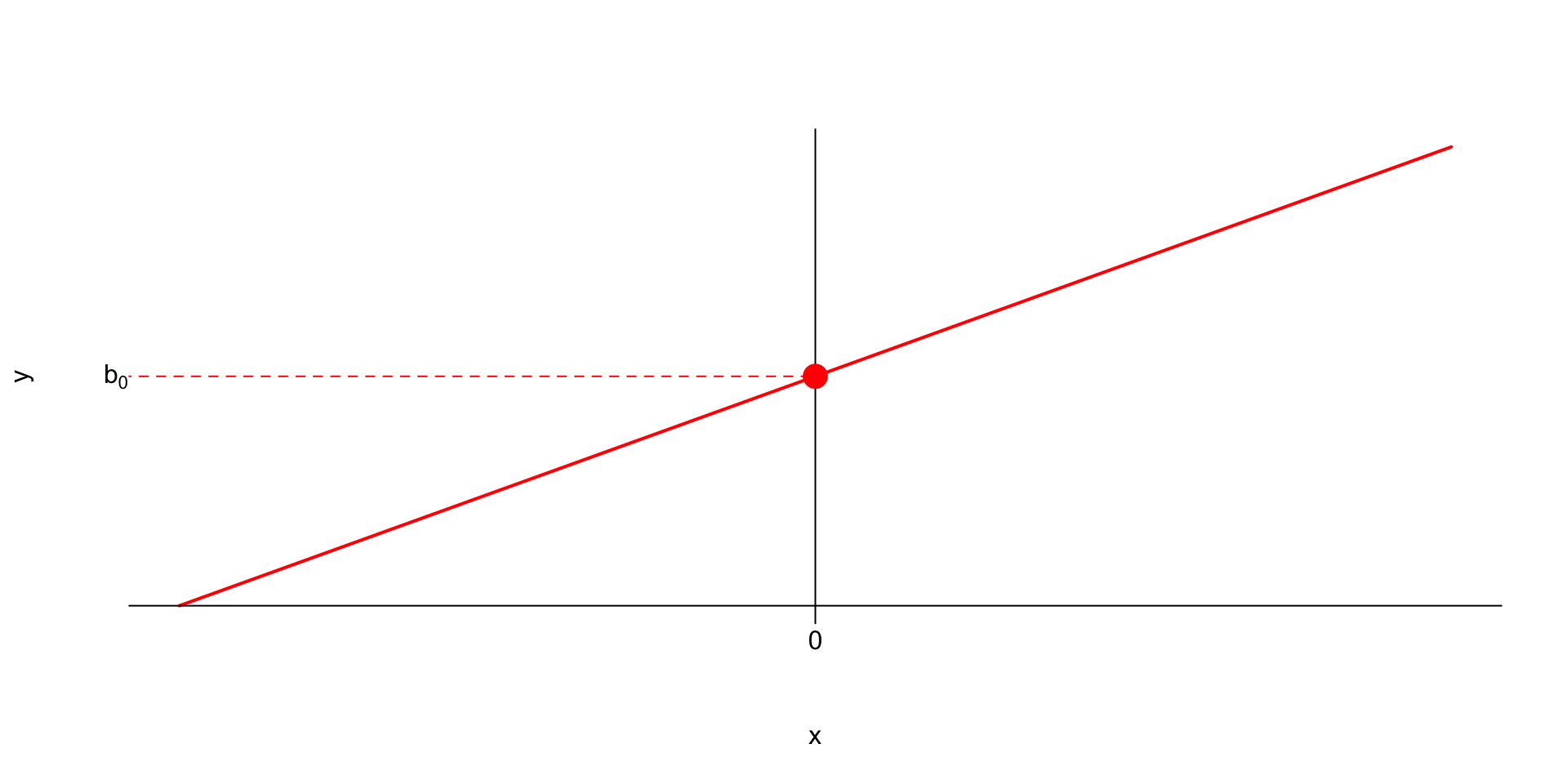
It’s the model’s prediction for \(y\) when \(x=0\).
Plug in \(x=0\) and simplify:
\[ \hat{y}=b_0+b_1\cdot 0=b_0. \]
If \(x=0\), we predict \(y\) will be \(b_0\) on average.
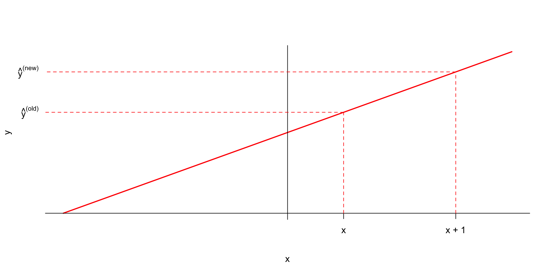
How does the prediction change when you change the input?
At \(x\), you predict:
\[ \hat{y}^{(\text{old})} = b_0+b_1x. \]
At \(x + 1\), you predict:
\[ \hat{y}^{(\text{new})} = b_0+b_1(x+1) = b_0+b_1x+b_0=\hat{y}^{(\text{old})}+b_1. \]
So when the predictor shifts from \(x\) to \(x+1\), the slope \(b_1\) tells you the additive adjustment you must make to go from the old prediction to the new one. It’s the same adjustment regardless the \(x\) you start from.
The “intercept” determines what the model predicts when x = 0.
Plug in \(x=0\) and simplify the formula:
\[ \hat{p}=\widehat{P(y=1\mid x = 0)}=\frac{e^{b_0+b_1\times 0}}{1+e^{b_0+b_1\times 0}}=\frac{e^{b_0}}{1+e^{b_0}}. \]
If \(x=0\), we predict that on average \(y=1\) with probability \(\frac{e^{b_0}}{1+e^{b_0}}\).
\[ \log\left(\frac{\hat{p}}{1-\hat{p}}\right) = -2.27 + 0.000272\times exclaim~mess \]
If exclaim_mess = 0, then
\[ \hat{p}=\widehat{P(y=1\mid x = 0)}=\frac{e^{-2.27}}{1+e^{-2.27}}\approx 0.09. \]
So, our model predicts that an email with no exclamation marks has a 9% probability of being spam.
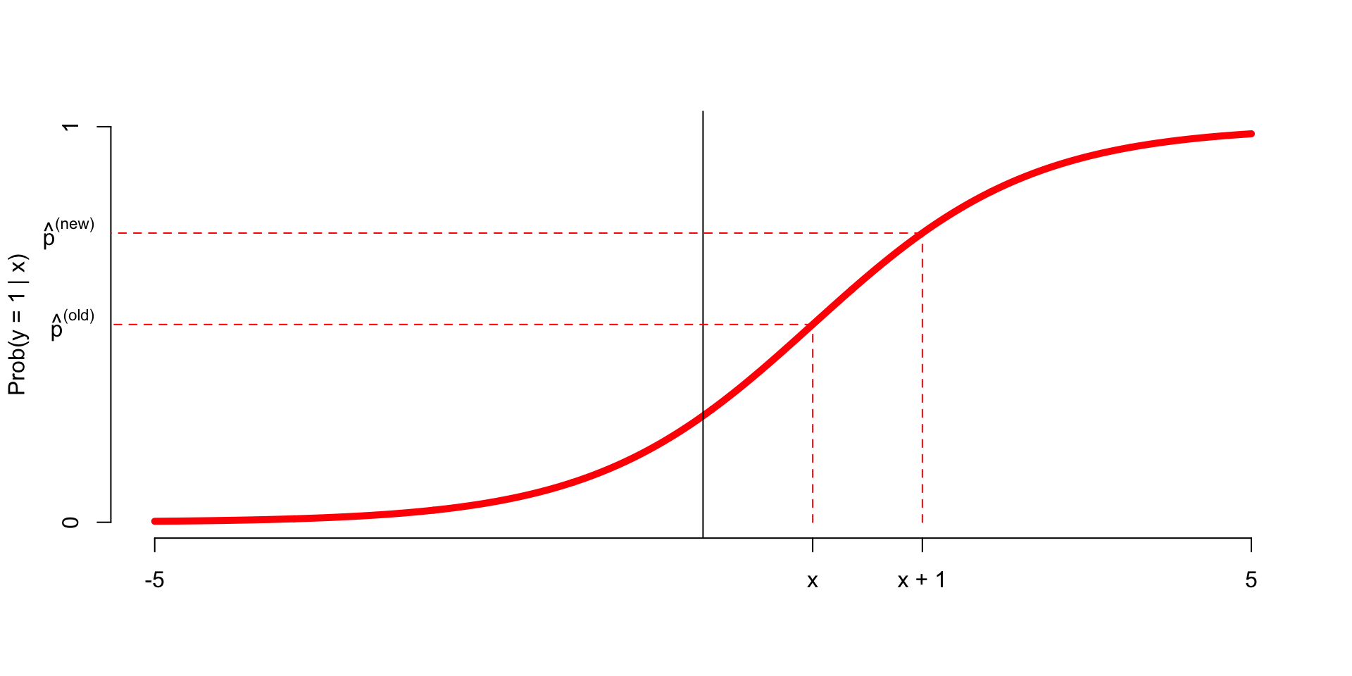
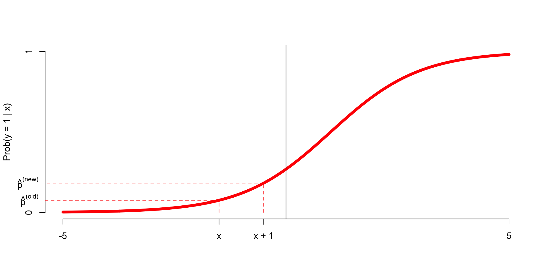
How does the prediction change when you change the input?
Does the adjustment depend on the \(x\) you’re starting from?
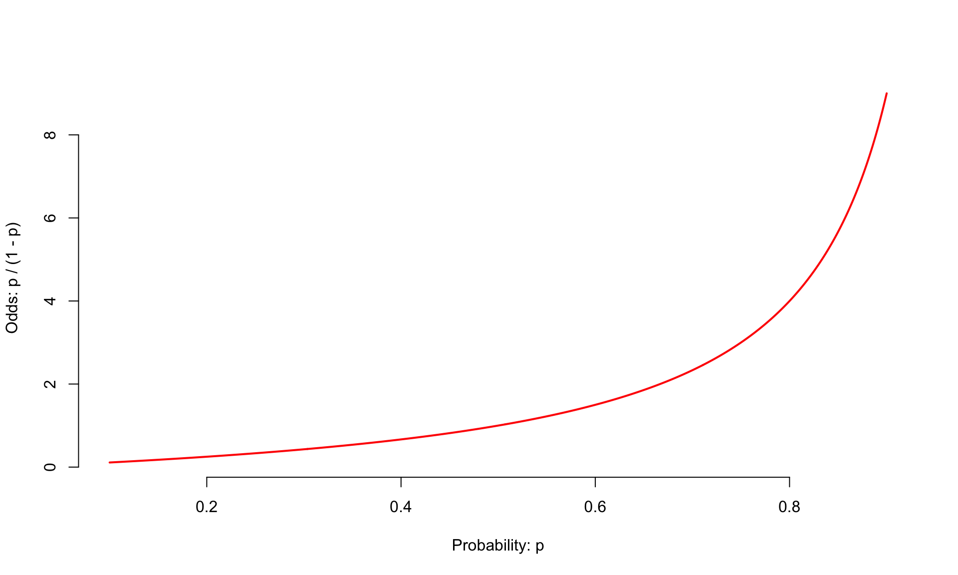
Probability:
\[ \hat{p} = \frac{e^{b_0+b_1x}}{1+e^{b_0+b_1x}}. \]
Odds:
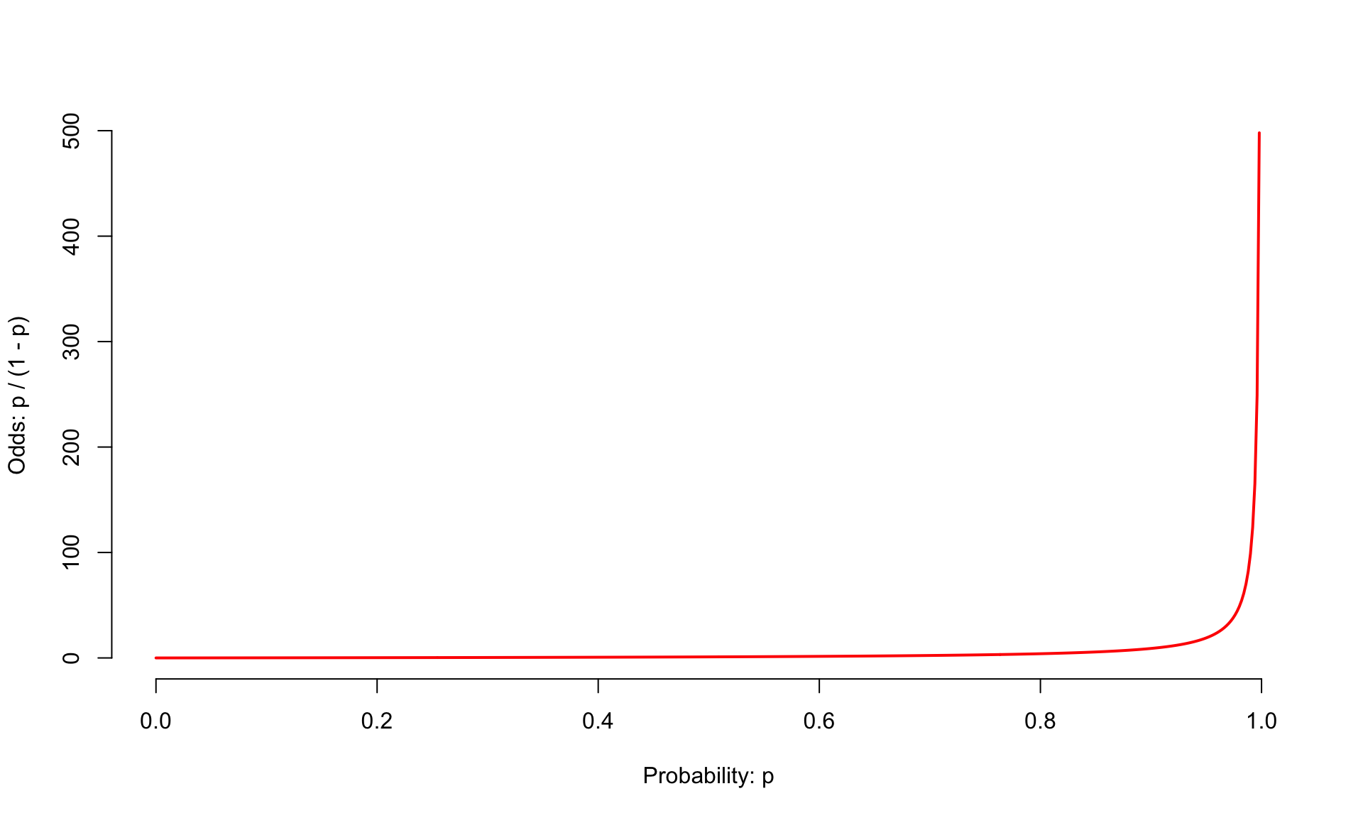
\[ \hat{o}=\frac{\widehat{p}}{1-\widehat{p}}=e^{b_0+b_1 x}. \]
Log-odds:
\[ \log\left(\hat{o}\right) = \log\left(\frac{\widehat{p}}{1-\widehat{p}}\right) = b_0+b_1x. \]
At \(x\), you predict:
\[ \log\left(\hat{o}^{(\text{old})}\right) = b_0+b_1x. \]
At \(x + 1\), you predict:
\[ \begin{aligned} \log\left(\hat{o}^{(\text{new})}\right) &= b_0+b_1(x+1)\\ &= b_0+b_1x+b_1 \\ &= \log\left(\hat{o}^{(\text{old})}\right)+b_1. \end{aligned} \]
Just like in linear regression, when the predictor shifts from \(x\) to \(x+1\), the “slope” \(b_1\) tell you the additive adjustment you must make to go from the old log-odds to the new log-odds. It’s the same adjustment regardless the \(x\) you start from.
At \(x\), you predict:
\[ \hat{o}^{(\text{old})} = e^{b_0+b_1x}. \]
At \(x + 1\), you predict:
\[ \hat{o}^{(\text{new})} = e^{b_0+b_1(x+1)} = e^{b_0+b_1x+b_1} = e^{b_0+b_1x}e^{b_1} = \hat{o}^{(\text{old})}\times e^{b_1} . \]
When the predictor shifts from \(x\) to \(x+1\), the transformed “slope” \(e^{b_1}\) tell you the multiplicative adjustment you must make to go from the old odds to the new odds. It’s the same adjustment regardless the \(x\) you start from.
We have this:
\[ \hat{o}^{(\text{new})} = \hat{o}^{(\text{old})}\times e^{b_1} . \]
\[ \log\left(\frac{\hat{p}}{1-\hat{p}}\right) = -2.27 + 0.000272\times exclaim~mess \]
If the email has an additional exclamation mark, we predict the odds of an email being spam to be higher by a multiplicative factor of \(e^{0.000272}\approx 1.000272\) on average.
At \(x\), you predict:
\[ \hat{p}^{(\text{old})} = \frac{e^{b_0+b_1x}}{1+e^{b_0+b_1x}} \]
At \(x + 1\), you predict:
\[ \hat{p}^{(\text{new})} = \frac{e^{b_0+b_1(x+1)}}{1+e^{b_0+b_1(x+1)}} \]
This one is tougher. You are not responsible for it, but if you really want to know, the math is relatively painless if you’re into that sort of thing:
How are \(\hat{p}^{(\text{old})}\) and \(\hat{p}^{(\text{new})}\) related?
Like this:
\[ \hat{p}^{(\text{new})} = \frac{e^{b_1}\hat{p}^{(\text{old})}}{1-\hat{p}^{(\text{old})}+e^{b_1}\hat{p}^{(\text{old})}} \]
The adjustment depends on the \(x\) you are starting from, just like we saw in the picture.
| Version | equation | Friendly LHS? | Friendly RHS? |
|---|---|---|---|
| Probability: (0, 1) | \[\hat{p}=\frac{e^{b_0+b_1x}}{1+e^{b_0+b_1x}}\] | ✅ | ❌ |
| Odds: \((0,\,\infty)\) | \[\hat{o}=\frac{\hat{p}}{1-\hat{p}}=e^{b_0+b_1x}\] | 🥴 | 🥴 |
| Log-odds: \((-\infty,\,\infty)\) | \[\log(\hat{o})=b_0+b_1x\] | ❌ | ✅ |
Take your pick depending on what you’re trying to do.
We have this model:
\[ \hat{p}=\widehat{\text{Prob}(y=1\mid x)} = \frac{e^{b_0+b_1x}}{1+e^{b_0+b_1x}}. \]
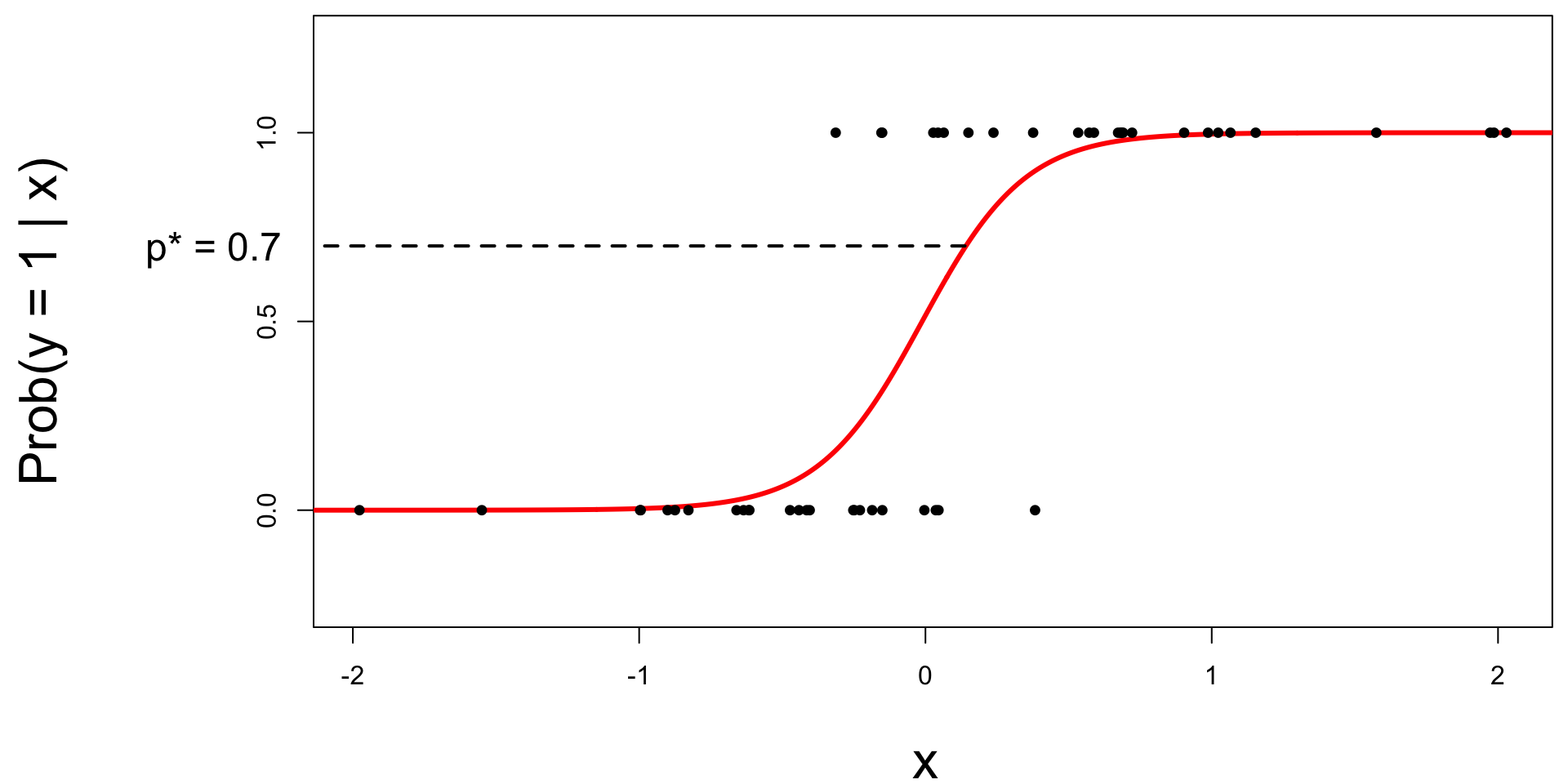
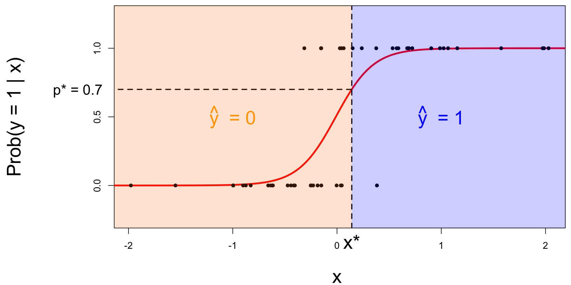
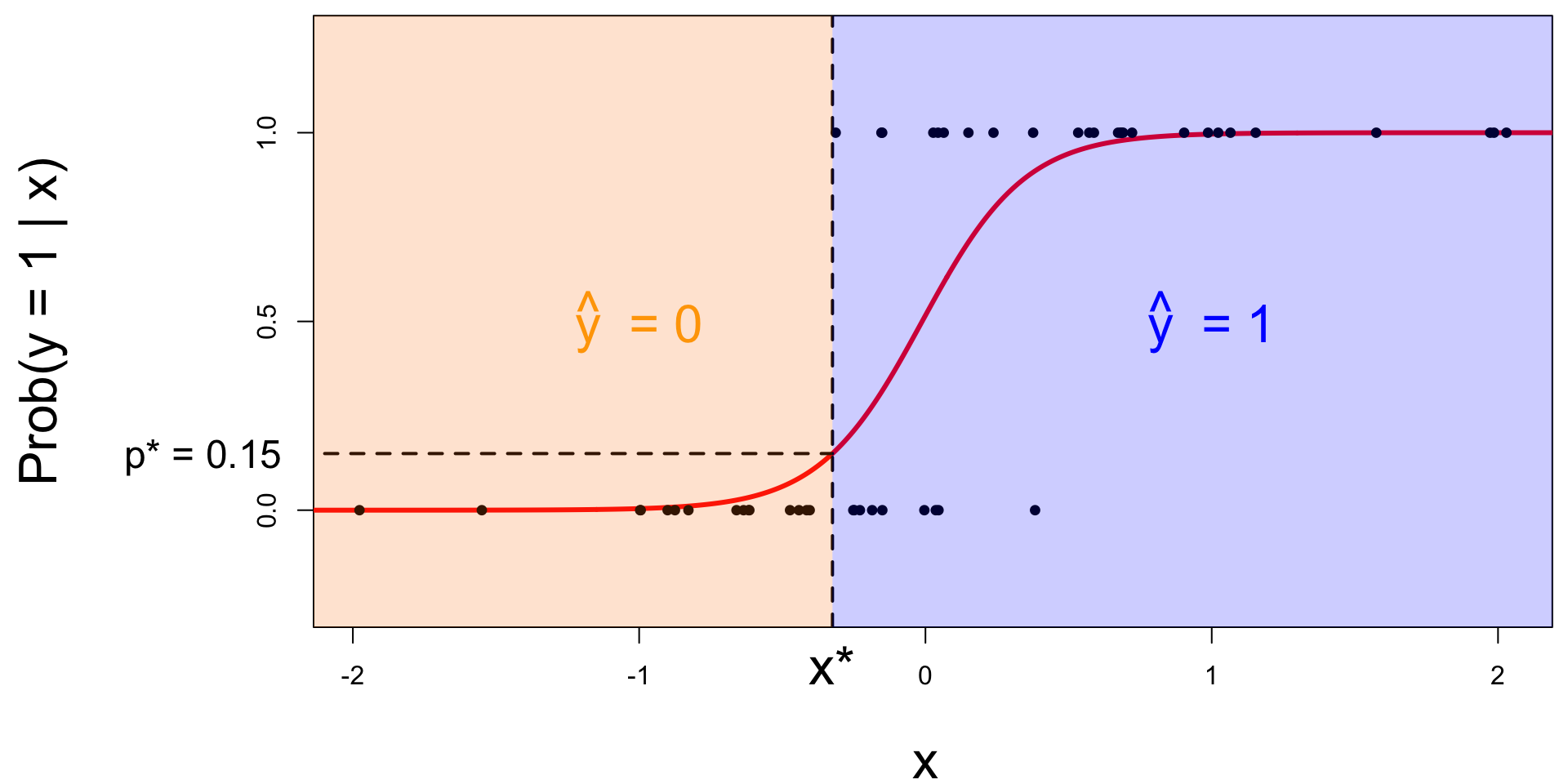
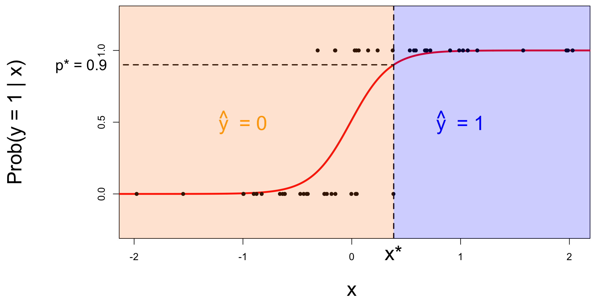
Given \(x\), we predict the probability that \(y=1\). But…so? If you hand me \(x\), is \(y=1\) or not? How can we use this model to produce a concrete prediction for the value of \(y\)? Behold…
Select a number \(0 < p^* < 1\):
Solve for the x-value that matches the threshold:
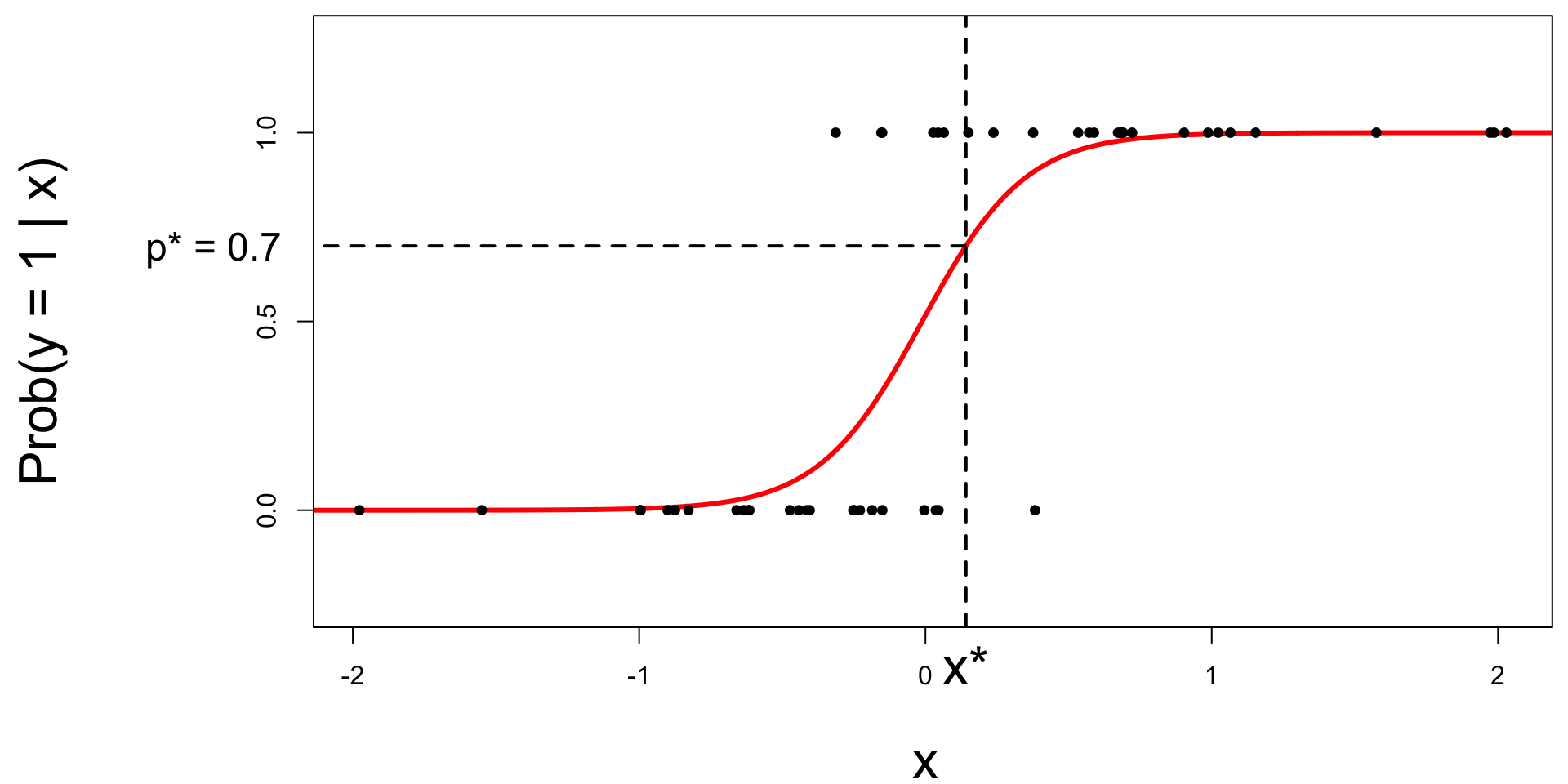
A new person shows up with \(x_{\text{new}}\). Which side of the boundary are they on?
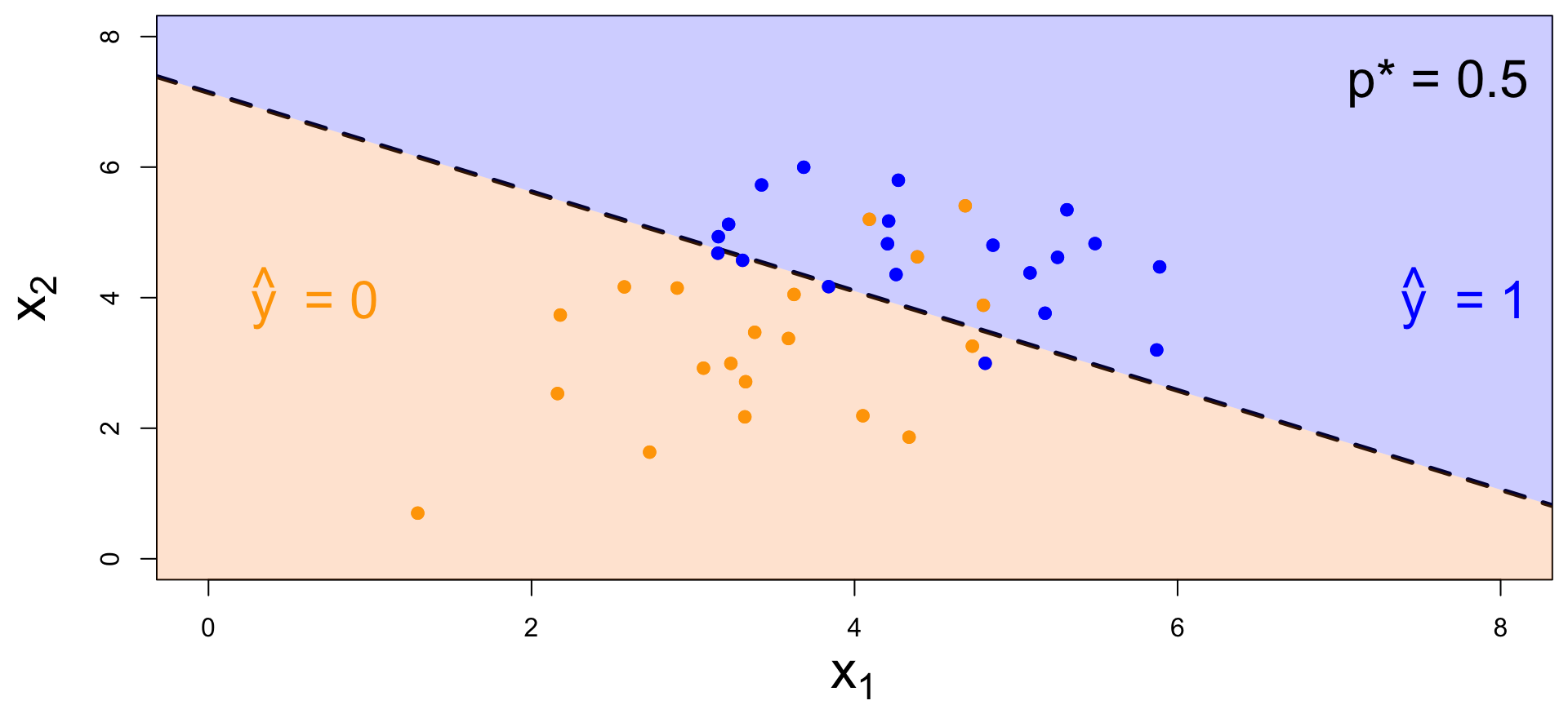
Two numerical predictors and one binary response:
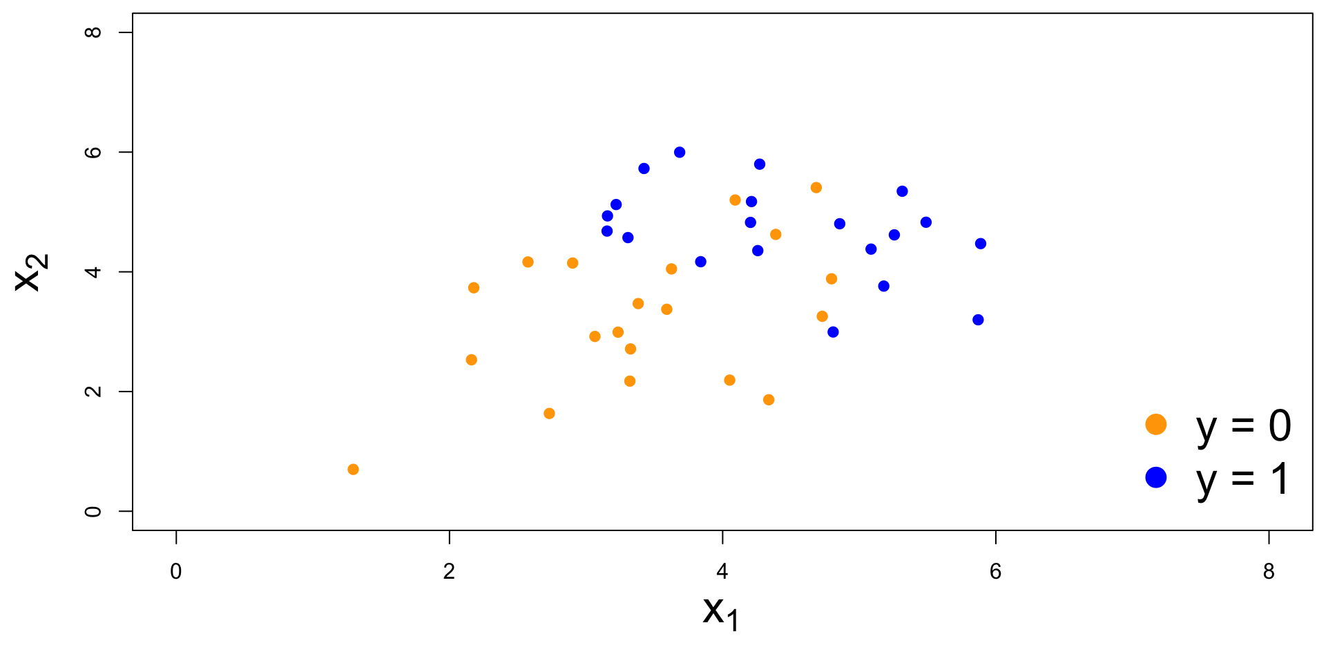
For the log-odds, a multiple linear regression:
\[ \log\left(\frac{p}{1-p}\right) = \beta_0+\beta_1x_1+\beta_2x_2+...+\beta_mx_m. \] On the probability scale:
\[ \text{Prob}(y = 1 \mid x) = \frac{e^{\beta_0+\beta_1x_1+\beta_2x_2+...+\beta_mx_m}}{1+e^{\beta_0+\beta_1x_1+\beta_2x_2+...+\beta_mx_m}}. \]
It’s linear! Consider two numerical predictors:
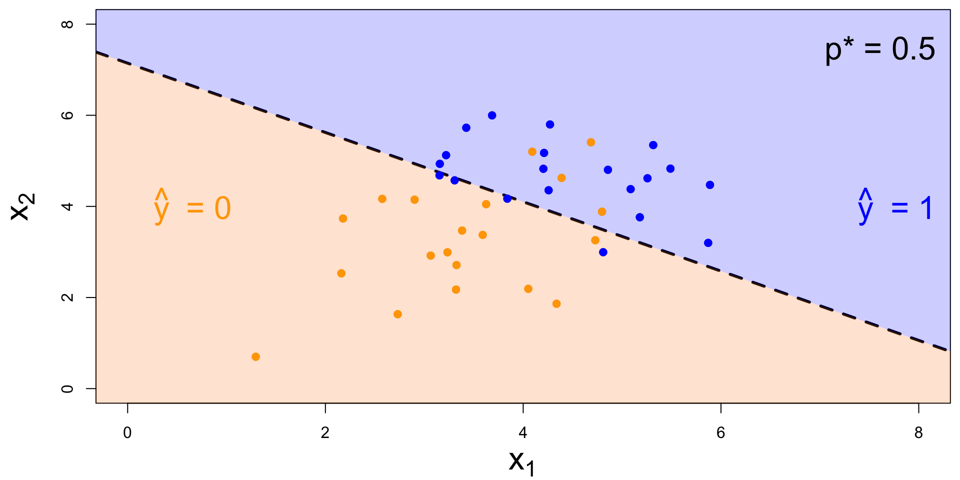
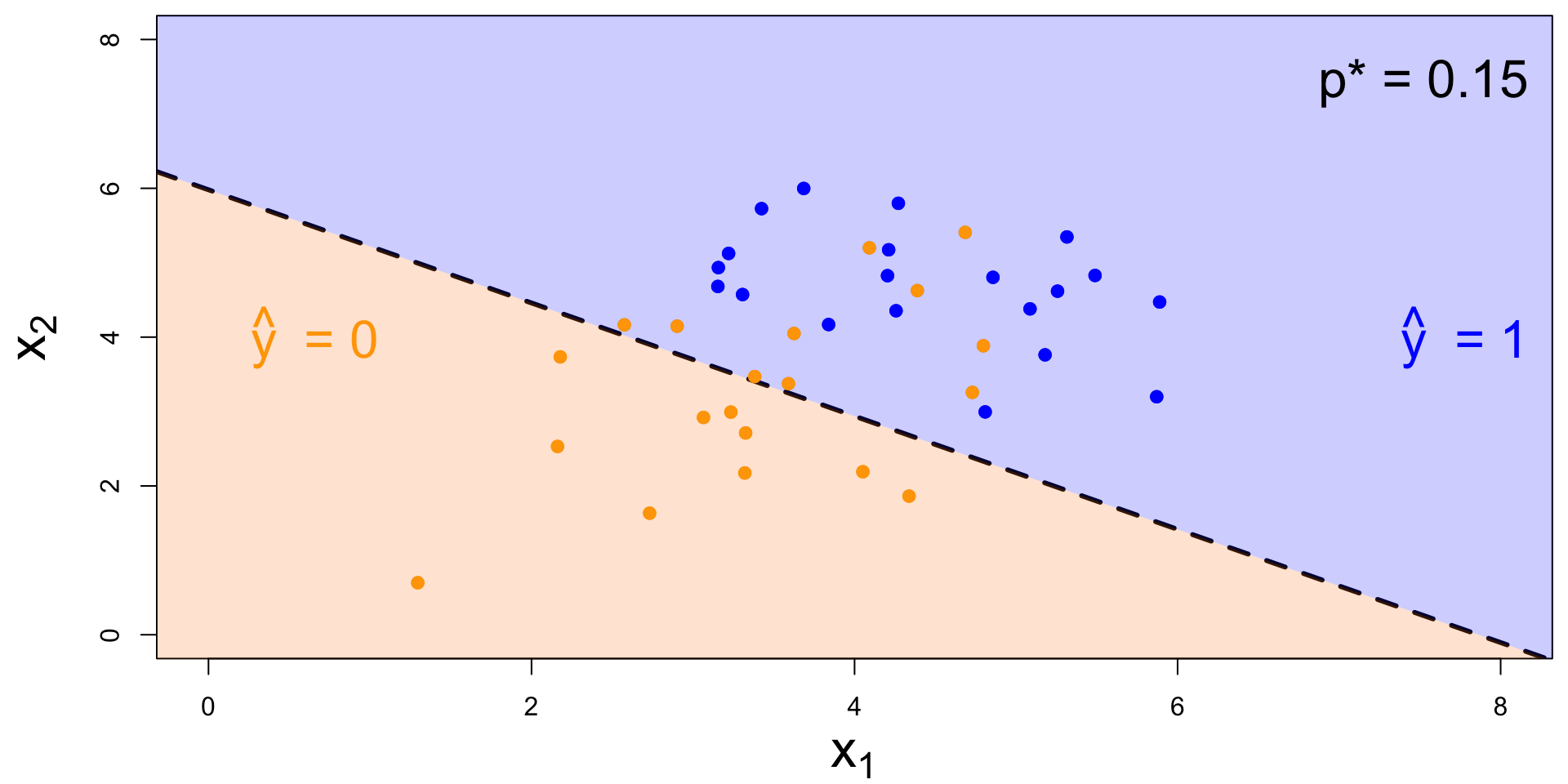
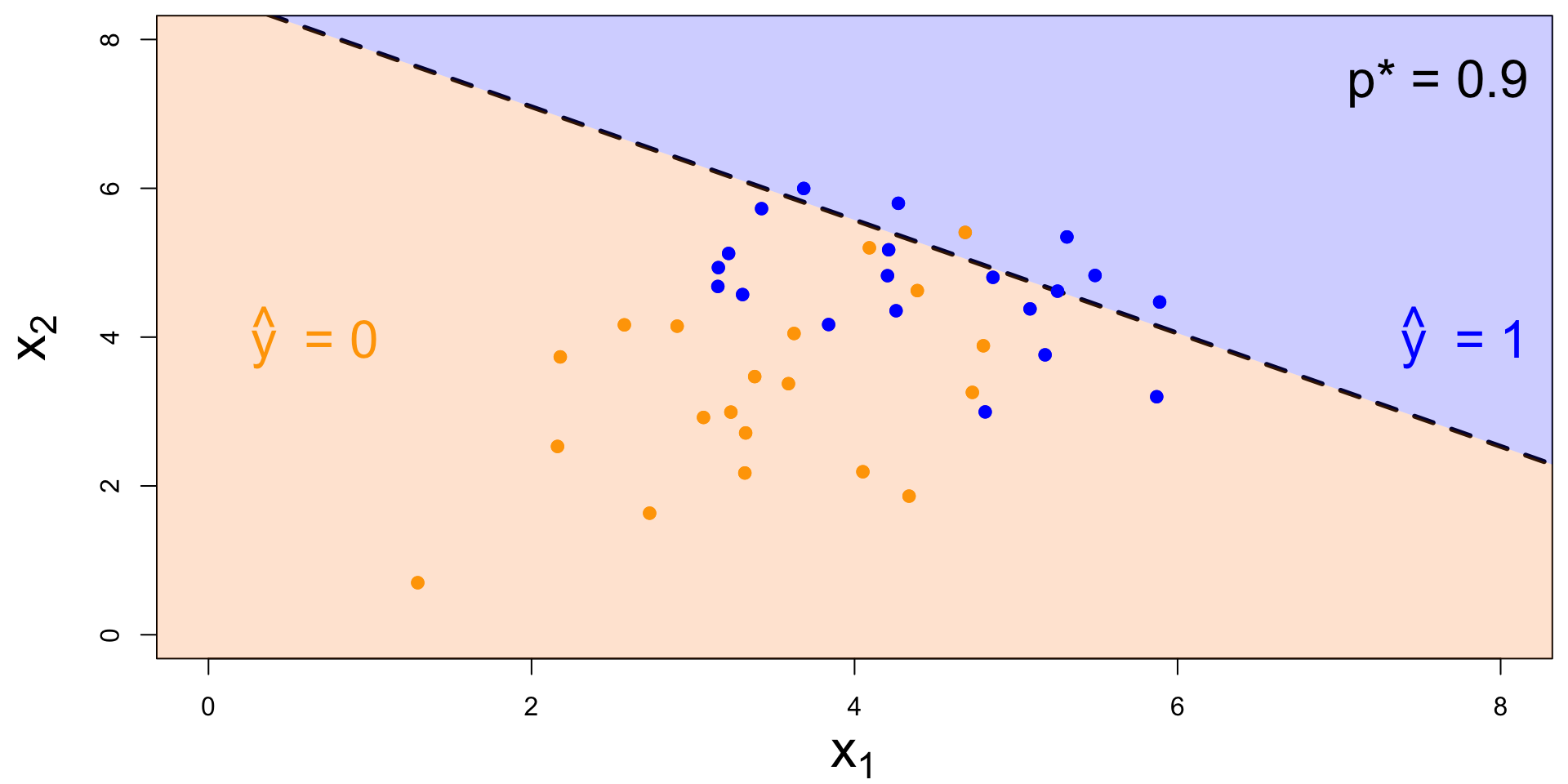
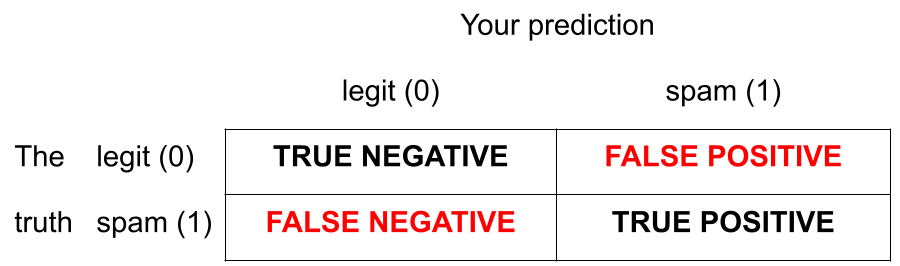
To balance out the two kinds of errors:
Set p* = 0
Set p* = 1
You pick a threshold in between to strike a balance. The exact number depends on context.