Model selection

Lecture 8

John Zito

Duke University
STA 101 Fall 2026

2026-09-24

Last time: $R^2$ for real

$R^2$ measures a model’s goodness-of-fit;
$R^2$ is defined as the proportion of variation in the response variable explained by the model. So, one minus the proportion of variation unexplained:

\[ R^2=1-\frac{\text{var}(e_i)}{\text{var}(y_i)}. \]

$R^2=1$ indicates perfect fit, $R^2=0$ indicates horrific fit, and everything in between. Like a “Rotten Tomatoes score” for your model.

Last time: penguins

We saw five different models all trying to predict the same thing:

bm_fl_fit <- linear_reg() |>
  fit(body_mass_g ~ flipper_length_mm, penguins)

bm_island_fit <- linear_reg() |>
  fit(body_mass_g ~ island, penguins)

bm_fl_island_fit <- linear_reg() |>
  fit(body_mass_g ~ flipper_length_mm + island, penguins)

bm_fl_island_int_fit <- linear_reg() |>
  fit(body_mass_g ~ flipper_length_mm * island, penguins)

bm_fl_bl_fit <- linear_reg() |>
  fit(body_mass_g ~ flipper_length_mm + bill_length_mm, penguins)

Model selection

Question: Given many competing models for the same response, which model is “best”? What does that even mean?

Answer: Assign a “quality score” to each model, and pick the model with the best score:

Model	Score	Verdict
Simple	0.1	❌
Additive	0.5	✅
Interaction	0.48	❌

Variable selection: all of our models were linear, and they differed only by which predictor variables are included. By ranking models by quality score and picking the “best” one, we can determine which predictors are the “most important” to include.

Selection criteria

This is a big area of statistical research. There are loads of “quality scores” you could consider, and they prioritize different things: predictive accuracy, goodness-of-fit, simplicity, fairness, etc.

$R^2$;
adjusted $R^2$;
Akaike Information criterion (AIC);
Bayesian information criterion (BIC);
… so many more

We won’t go into detail, but you will if you keep studying statistics.

`tidymodels` reports many of these for free

bm_fl_fit |>
  glance() |>
  select(r.squared, adj.r.squared, AIC, BIC)

# A tibble: 1 × 4
  r.squared adj.r.squared   AIC   BIC
      <dbl>         <dbl> <dbl> <dbl>
1     0.759         0.758 5063. 5074.

$R^2$’s dirty little secret

$R^2$ gives participation trophies. It always goes up when you add any new variable to the model, even if that variable is worthless.

Adding a phony variable

The original model fit:

linear_reg() |>
  fit(body_mass_g ~ flipper_length_mm, penguins) |>
  glance() |>
  pull(r.squared)

[1] 0.7589925

Add a predictor that is literally just a bunch of random numbers:

noisy_penguins <- penguins |>
  mutate(
    bullshit = rnorm(nrow(penguins))
  )

linear_reg() |>
  fit(body_mass_g ~ flipper_length_mm + bullshit, noisy_penguins) |>
  glance() |>
  pull(r.squared)

[1] 0.7600283

Adjusted $R^2$

Because vanilla $R^2$ blithely rewards the addition of any variable, no matter how meaningless, you shouldn’t use it for model selection. Instead, use adjusted $R^2$. The formula is in the textbook if you’re dying to know, but here’s the tea:

adjusted $R^2$ penalizes the inclusion of unnecessary predictors;
It prioritizes a parsimonious model:
- a model that fits/predicts well, and…
- a model that’s not too complicated (so our pea brains can still understand it);
Occam’s razor!

For the penguins

bm_fl_fit |> glance() |>
  pull(adj.r.squared)

[1] 0.7582837

bm_island_fit |> glance() |>
  pull(adj.r.squared)

[1] 0.3899995

bm_fl_island_fit |> glance() |>
  pull(adj.r.squared)

[1] 0.7722296

bm_fl_island_int_fit |> glance() |>
  pull(adj.r.squared)

[1] 0.7825604

bm_fl_bl_fit |> glance() |>
  pull(adj.r.squared)

[1] 0.7585415

Which model is “best”?

Balancing fit and complexity

More complex models (i.e., models with more predictors) tend to fit the data at hand better, but may not generalize well to new data.
Model selection criteria, like adjusted $R^2$, help balance model fit and complexity to avoid overfitting by penalizing models with more predictors.

Overfitting

Overfitting occurs when a model captures not only the underlying relationship between predictors and outcome but also the random noise in the data;
Overfitted models tend to perform well on the observed data but poorly on new, unseen data.
- Good news: We have techniques to detect and prevent overfitting;
- Bad news: We won’t get into those until next week.

Back to variable selection

Given a set of competing models, all trying to predict the same response, we can line ’em up, compute adjusted $R^2$ for each model, and then pick the model with the highest score.

Easy, right?

Listing out all the possible models

The penguins dataset has $p=6$ variables apart from body mass: species, island, bill length, bill depth, flipper length, and sex;
How many models is that (ignoring the possibility of interaction, which makes things worse):
- 1 “empty” model: include no predictors;
- 6 “simple” models: include only one predictor;
- 15 two-predictor models;
- 20 three-predictor models;
- 15 four-predictor models;
- 6 five-predictor models;
- 1 “full” model: include all predictors.
That’s $2^6=64$ models in total you have to consider. Not the end of the world if you have a computer, but it gets worse…

Combinatorial explosion

If you have $p$ candidate predictors, then the set of all possible subsets you could include in a model grows very quickly;
In the “big data” era, 100 predictors is amateur hour, so it becomes infeasible to fit every possible model;
It pays to “search” through the space of models in a smarter, less brute-force way.

$p$	# of models = $2^p$
2	4
5	32
10	1024
20	1048576
30	1073741824
40	$\approx 1.098\times 10^{12}$
50	$\approx 1.13\times 10^{15}$
100	$\approx 1.27\times 10^{30}$

Backward elimination

Start with the full model (the model that includes all potential predictor variables). Variables are eliminated one-at-a-time from the model until we cannot improve the model any further.

Procedure:

Start with a model that has all predictors we consider and compute the adjusted $R^2$.
Next fit every possible model with 1 fewer predictor.
Compare adjusted $R^2$s to select the best model (highest adjusted $R^2$) with 1 fewer predictor.
Repeat steps 2 and 3 until adjusted $R^2$ no longer increases.

Example: recall the cars

mtcars

                     mpg cyl  disp  hp drat    wt  qsec vs am gear carb
Mazda RX4           21.0   6 160.0 110 3.90 2.620 16.46  0  1    4    4
Mazda RX4 Wag       21.0   6 160.0 110 3.90 2.875 17.02  0  1    4    4
Datsun 710          22.8   4 108.0  93 3.85 2.320 18.61  1  1    4    1
Hornet 4 Drive      21.4   6 258.0 110 3.08 3.215 19.44  1  0    3    1
Hornet Sportabout   18.7   8 360.0 175 3.15 3.440 17.02  0  0    3    2
Valiant             18.1   6 225.0 105 2.76 3.460 20.22  1  0    3    1
Duster 360          14.3   8 360.0 245 3.21 3.570 15.84  0  0    3    4
Merc 240D           24.4   4 146.7  62 3.69 3.190 20.00  1  0    4    2
Merc 230            22.8   4 140.8  95 3.92 3.150 22.90  1  0    4    2
Merc 280            19.2   6 167.6 123 3.92 3.440 18.30  1  0    4    4
Merc 280C           17.8   6 167.6 123 3.92 3.440 18.90  1  0    4    4
Merc 450SE          16.4   8 275.8 180 3.07 4.070 17.40  0  0    3    3
Merc 450SL          17.3   8 275.8 180 3.07 3.730 17.60  0  0    3    3
Merc 450SLC         15.2   8 275.8 180 3.07 3.780 18.00  0  0    3    3
Cadillac Fleetwood  10.4   8 472.0 205 2.93 5.250 17.98  0  0    3    4
Lincoln Continental 10.4   8 460.0 215 3.00 5.424 17.82  0  0    3    4
Chrysler Imperial   14.7   8 440.0 230 3.23 5.345 17.42  0  0    3    4
Fiat 128            32.4   4  78.7  66 4.08 2.200 19.47  1  1    4    1
Honda Civic         30.4   4  75.7  52 4.93 1.615 18.52  1  1    4    2
Toyota Corolla      33.9   4  71.1  65 4.22 1.835 19.90  1  1    4    1
Toyota Corona       21.5   4 120.1  97 3.70 2.465 20.01  1  0    3    1
Dodge Challenger    15.5   8 318.0 150 2.76 3.520 16.87  0  0    3    2
AMC Javelin         15.2   8 304.0 150 3.15 3.435 17.30  0  0    3    2
Camaro Z28          13.3   8 350.0 245 3.73 3.840 15.41  0  0    3    4
Pontiac Firebird    19.2   8 400.0 175 3.08 3.845 17.05  0  0    3    2
Fiat X1-9           27.3   4  79.0  66 4.08 1.935 18.90  1  1    4    1
Porsche 914-2       26.0   4 120.3  91 4.43 2.140 16.70  0  1    5    2
Lotus Europa        30.4   4  95.1 113 3.77 1.513 16.90  1  1    5    2
Ford Pantera L      15.8   8 351.0 264 4.22 3.170 14.50  0  1    5    4
Ferrari Dino        19.7   6 145.0 175 3.62 2.770 15.50  0  1    5    6
Maserati Bora       15.0   8 301.0 335 3.54 3.570 14.60  0  1    5    8
Volvo 142E          21.4   4 121.0 109 4.11 2.780 18.60  1  1    4    2

Example: recall the cars

(AIC is an alternative selection criterion. Lower is better.)

backward_model <- lm(mpg ~ ., data = mtcars)

backward_model <- stats::step(backward_model, direction = "backward")

Start:  AIC=70.9
mpg ~ cyl + disp + hp + drat + wt + qsec + vs + am + gear + carb

       Df Sum of Sq    RSS    AIC
- cyl   1    0.0799 147.57 68.915
- vs    1    0.1601 147.66 68.932
- carb  1    0.4067 147.90 68.986
- gear  1    1.3531 148.85 69.190
- drat  1    1.6270 149.12 69.249
- disp  1    3.9167 151.41 69.736
- hp    1    6.8399 154.33 70.348
- qsec  1    8.8641 156.36 70.765
<none>              147.49 70.898
- am    1   10.5467 158.04 71.108
- wt    1   27.0144 174.51 74.280

Step:  AIC=68.92
mpg ~ disp + hp + drat + wt + qsec + vs + am + gear + carb

       Df Sum of Sq    RSS    AIC
- vs    1    0.2685 147.84 66.973
- carb  1    0.5201 148.09 67.028
- gear  1    1.8211 149.40 67.308
- drat  1    1.9826 149.56 67.342
- disp  1    3.9009 151.47 67.750
- hp    1    7.3632 154.94 68.473
<none>              147.57 68.915
- qsec  1   10.0933 157.67 69.032
- am    1   11.8359 159.41 69.384
- wt    1   27.0280 174.60 72.297

Step:  AIC=66.97
mpg ~ disp + hp + drat + wt + qsec + am + gear + carb

       Df Sum of Sq    RSS    AIC
- carb  1    0.6855 148.53 65.121
- gear  1    2.1437 149.99 65.434
- drat  1    2.2139 150.06 65.449
- disp  1    3.6467 151.49 65.753
- hp    1    7.1060 154.95 66.475
<none>              147.84 66.973
- am    1   11.5694 159.41 67.384
- qsec  1   15.6830 163.53 68.200
- wt    1   27.3799 175.22 70.410

Step:  AIC=65.12
mpg ~ disp + hp + drat + wt + qsec + am + gear

       Df Sum of Sq    RSS    AIC
- gear  1     1.565 150.09 63.457
- drat  1     1.932 150.46 63.535
<none>              148.53 65.121
- disp  1    10.110 158.64 65.229
- am    1    12.323 160.85 65.672
- hp    1    14.826 163.35 66.166
- qsec  1    26.408 174.94 68.358
- wt    1    69.127 217.66 75.350

Step:  AIC=63.46
mpg ~ disp + hp + drat + wt + qsec + am

       Df Sum of Sq    RSS    AIC
- drat  1     3.345 153.44 62.162
- disp  1     8.545 158.64 63.229
<none>              150.09 63.457
- hp    1    13.285 163.38 64.171
- am    1    20.036 170.13 65.466
- qsec  1    25.574 175.67 66.491
- wt    1    67.572 217.66 73.351

Step:  AIC=62.16
mpg ~ disp + hp + wt + qsec + am

       Df Sum of Sq    RSS    AIC
- disp  1     6.629 160.07 61.515
<none>              153.44 62.162
- hp    1    12.572 166.01 62.682
- qsec  1    26.470 179.91 65.255
- am    1    32.198 185.63 66.258
- wt    1    69.043 222.48 72.051

Step:  AIC=61.52
mpg ~ hp + wt + qsec + am

       Df Sum of Sq    RSS    AIC
- hp    1     9.219 169.29 61.307
<none>              160.07 61.515
- qsec  1    20.225 180.29 63.323
- am    1    25.993 186.06 64.331
- wt    1    78.494 238.56 72.284

Step:  AIC=61.31
mpg ~ wt + qsec + am

       Df Sum of Sq    RSS    AIC
<none>              169.29 61.307
- am    1    26.178 195.46 63.908
- qsec  1   109.034 278.32 75.217
- wt    1   183.347 352.63 82.790

Foreward stepwise regression

Forward stepwise regression is the reverse of the backward elimination technique. Instead, of eliminating variables one-at-a-time, we start from an “empty model” and we add variables one-at-a-time until we cannot find any variables that improve the model any further.

Procedure:

Start with a model that has no predictors.
Next fit every possible model with 1 additional predictor and calculate adjusted $R^2$ of each model.
Compare adjusted $R^2$ values to select the best model (highest adjusted $R^2$) with 1 additional predictor.
Repeat steps 2 and 3 until adjusted $R^2$ no longer increases.

A new application

A girl’s best friend

A game

10-carat old mine brilliant-cut diamond
58 facets
Est. at $550K - $1M

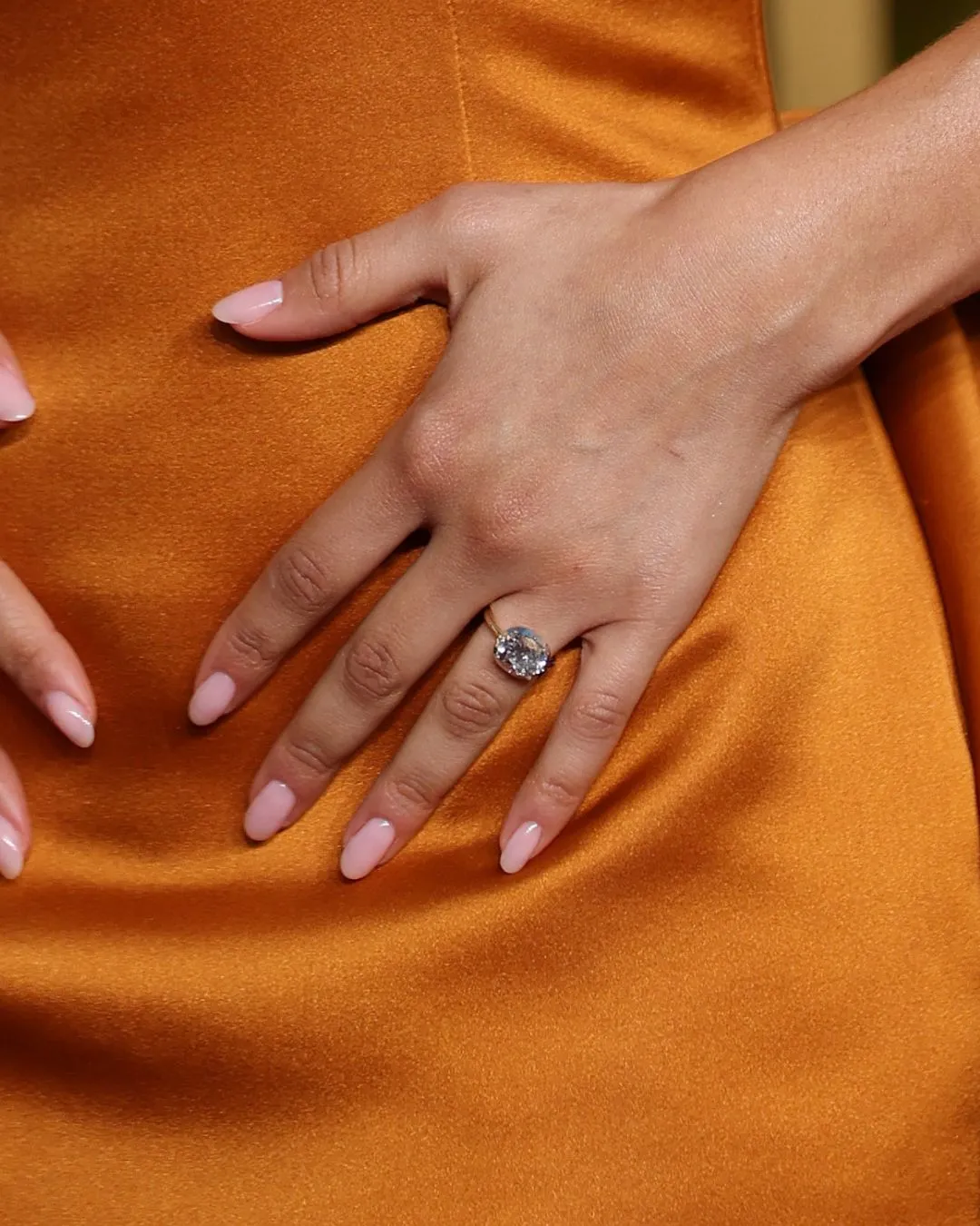
5-carat antique cushion-cut diamond
$280,000 price tag

Est. 30-40-carat high color center diamond
1-carat oval side stones
Est. value upwards of $3M

The 4 Cs

When evaluating a diamond, jewelers typically focus on four key characteristics known as the 4 Cs:

Carat — How big is it?
Cut — How much does it sparkle?
Clarity — How flawless is it?
Color — How colorless is it?

The 4 Cs are the primary factors that determine a diamond’s value.

What do these things mean?

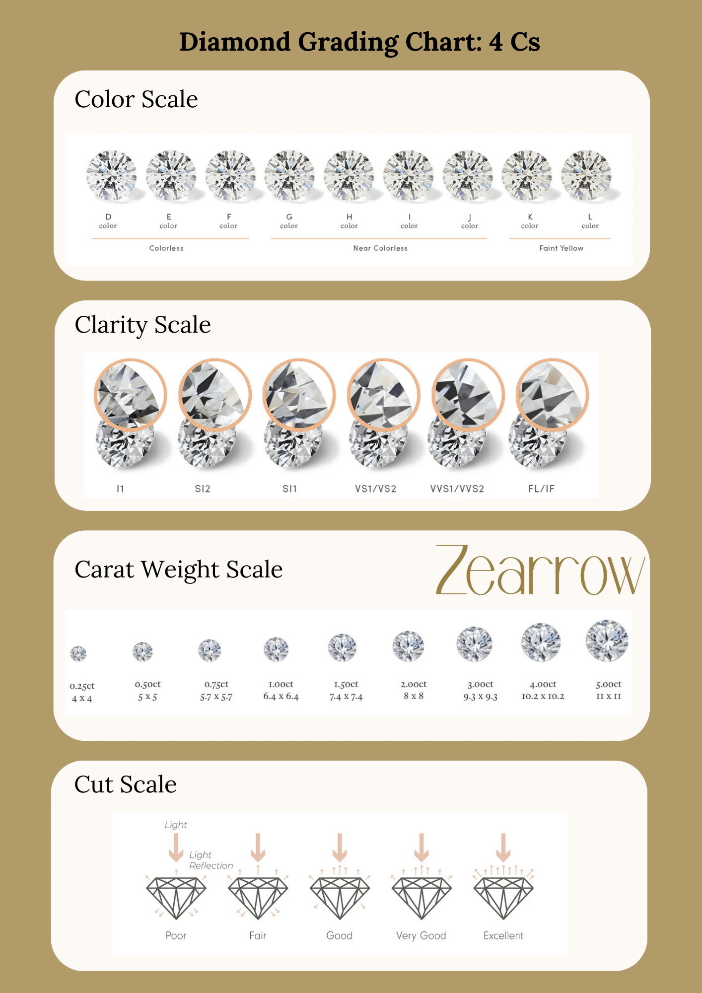
What do these things mean?

For example:

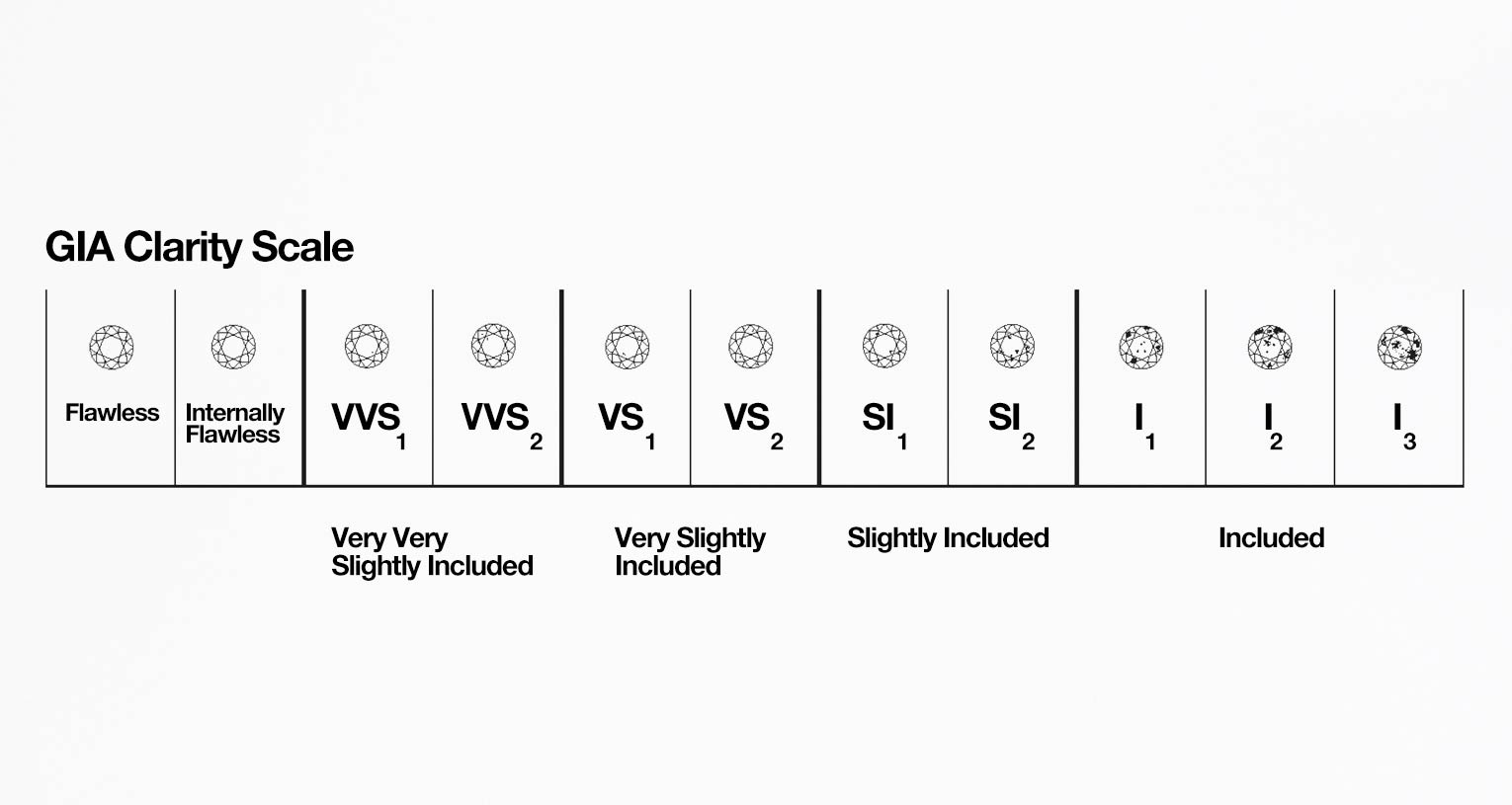
We have some data!

diamonds

# A tibble: 5,000 × 7
   price carat cut       color clarity length_mm width_mm
   <dbl> <dbl> <fct>     <fct> <fct>       <dbl>    <dbl>
 1  3867  0.9  Ideal     I     VS           6.13     6.18
 2 12048  2.01 Ideal     J     SI           8.08     8.03
 3   878  0.41 Very Good F     SI           4.73     4.69
 4  4325  0.68 Ideal     D     VVS          5.66     5.69
 5   401  0.3  Ideal     E     SI           4.33     4.35
 6  5504  1.19 Ideal     D     SI           6.91     6.89
 7  1767  0.63 Good      H     VS           5.47     5.56
 8  4704  1.02 Very Good G     SI           6.36     6.4 
 9  1121  0.52 Ideal     F     SI           5.17     5.2 
10  2137  0.7  Very Good H     VS           5.58     5.62
# ℹ 4,990 more rows

Now, off to your container!

Model selection

Last time: \(R^2\) for real

Last time: penguins

Model selection

Selection criteria

`tidymodels` reports many of these for free

\(R^2\)’s dirty little secret

Adding a phony variable

Adjusted \(R^2\)

For the penguins

Balancing fit and complexity

Overfitting

Back to variable selection

Listing out all the possible models

Combinatorial explosion

Backward elimination

Example: recall the cars

Example: recall the cars

Foreward stepwise regression

A new application

A girl’s best friend

A game

The 4 Cs

What do these things mean?

What do these things mean?

We have some data!

Now, off to your container!

\(p\)	# of models = \(2^p\)
2	4
5	32
10	1024
20	1048576
30	1073741824
40	\(\approx 1.098\times 10^{12}\)
50	\(\approx 1.13\times 10^{15}\)
100	\(\approx 1.27\times 10^{30}\)

Model selection

Last time: \(R^2\) for real

Last time: penguins

Model selection

Selection criteria

tidymodels reports many of these for free

\(R^2\)’s dirty little secret

Adding a phony variable

Adjusted \(R^2\)

For the penguins

Balancing fit and complexity

Overfitting

Back to variable selection

Listing out all the possible models

Combinatorial explosion

Backward elimination

Example: recall the cars

Example: recall the cars

Foreward stepwise regression

A new application

A girl’s best friend

A game

The 4 Cs

What do these things mean?

What do these things mean?

We have some data!

Now, off to your container!

`tidymodels` reports many of these for free