# A tibble: 2 × 5
  term              estimate std.error statistic   p.value
  <chr>                <dbl>     <dbl>     <dbl>     <dbl>
1 (Intercept)        -5781.     306.       -18.9 5.59e- 55
2 flipper_length_mm 49.7 1.52 32.7 4.37e-107Goodness-of-fit
Lecture 7
John Zito
Duke University
STA 101 Fall 2026
2026-09-22
Recap: linear regression
Population model
Multiple linear regression captures the relationship between a numerical outcome \(Y\) and many numerical predictors \(X_1\), \(X_2\), …, \(X_p\):
\[\Large{Y = \beta_0 + \beta_1 X_1 + \beta_2 X_2 + ...+ \beta_p X_p+\epsilon}\]
- \(\beta_0\): True intercept of the relationship between the \(X_j\) and \(Y\)
- \(\beta_j\): True slope of the relationship between \(X_j\) and \(Y\)
- \(\epsilon\): Error (residual)
The model with the greek letters and the error term is the “true,” idealized, population relationship that we could access if we had infinite amounts of perfect data. But we don’t, so we have to settle for…
Estimated model
\[\Large{\hat{Y} = b_0 + b_1 X_1 + b_2 X_2 + ... + b_pX_p}\]
- \(b_j\): Estimated slope of the relationship between \(X_j\) and \(Y\);
- \(b_0\): your prediction for \(Y\) if all the predictors equal zero;
- No error term!
This is your best guess at the true regression function based on the noisy, meager, imperfect data you actually have access to. We still compute the \(b_j\) using the principle of least squares: pick the estimates that make the sum of squared residuals as small as possible.
Example: one numerical predictor
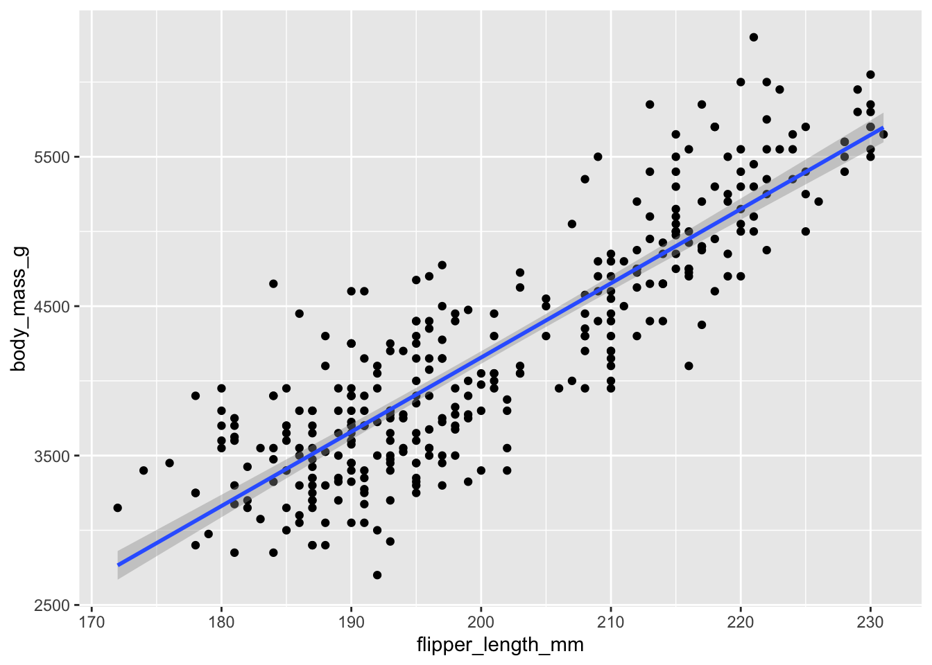
Example: one numerical predictor
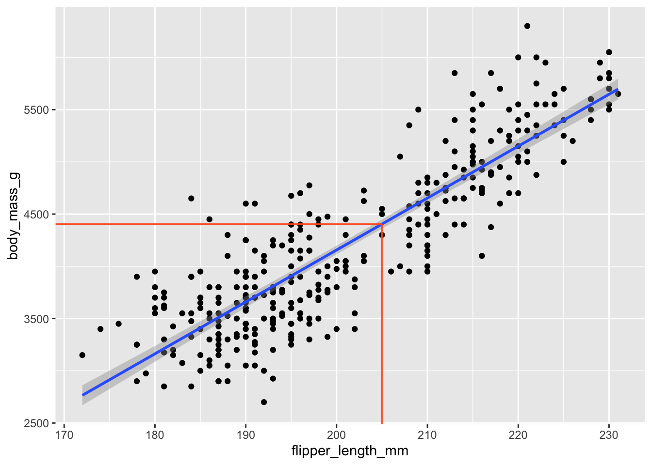
\[ \widehat{body~mass}=-5780.83+49.68\times flipper~length \]
Example: one numerical predictor
Example: “one categorical predictor”
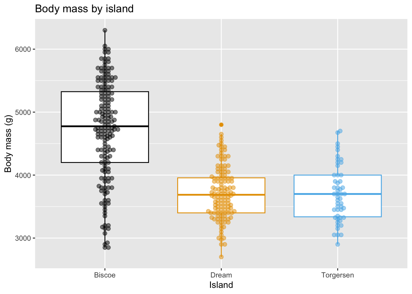
Example: “one categorical predictor”
This actually gets treated as multiple binary (0/1) predictors:
# A tibble: 3 × 5
  term            estimate std.error statistic   p.value
  <chr>              <dbl>     <dbl>     <dbl>     <dbl>
1 (Intercept)        4716.      48.5      97.3 8.93e-250
2 islandDream       -1003.      74.2     -13.5 1.42e- 33
3 islandTorgersen   -1010.     100.      -10.1 4.66e- 21
\[ \begin{aligned} \widehat{body~mass} = 4716 &- 1003 \times islandDream \\ &- 1010 \times islandTorgersen \end{aligned} \]
Example: “one categorical predictor”
It’s just a concise way of summarizing the within-group means of the response variable:
Example: numerical and categorical predictors
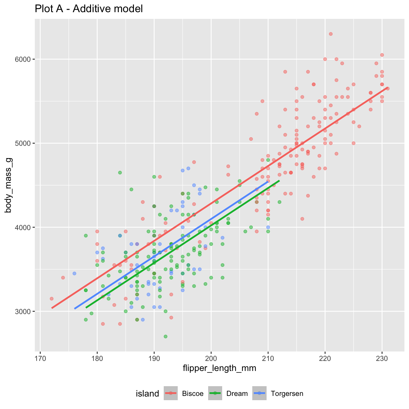
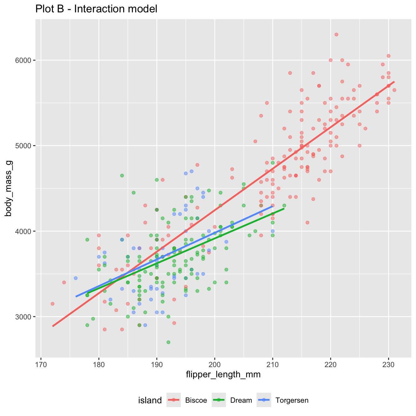
Example: numerical and categorical predictors
The additive model:
bm_fl_island_fit <- linear_reg() |>
  fit(body_mass_g ~ flipper_length_mm + island, data = penguins)

tidy(bm_fl_island_fit)
# A tibble: 4 × 5
term estimate std.error statistic p.value
<chr> <dbl> <dbl> <dbl> <dbl>
1 (Intercept) -4625. 392. -11.8 4.29e-27
2 flipper_length_mm 44.5 1.87 23.9 1.65e-74
3 islandDream -262. 55.0 -4.77 2.75e- 6
4 islandTorgersen -185. 70.3 -2.63 8.84e- 3\[ \begin{aligned} \widehat{body~mass} = -4625 &+ 44.5 \times flipper~length \\ &- 262 \times Dream \\ &- 185 \times Torgersen \end{aligned} \]
Example: numerical and categorical predictors
Change one character in the code, and you get the interaction model:
bm_fl_island_int_fit <- linear_reg() |>
  fit(body_mass_g ~ flipper_length_mm * island, data = penguins)

tidy(bm_fl_island_int_fit) |> select(term, estimate)
# A tibble: 6 × 2
term estimate
<chr> <dbl>
1 (Intercept) -5464.
2 flipper_length_mm 48.5
3 islandDream 3551.
4 islandTorgersen 3218.
5 flipper_length_mm:islandDream -19.4
6 flipper_length_mm:islandTorgersen -17.4\[ \begin{aligned} \widehat{body~mass} = -5464 &+ 48.5 \times flipper~length \\ &+ 3551 \times Dream \\ &+ 3218 \times Torgersen \\ &- 19.4 \times flipper~length*Dream \\ &- 17.4 \times flipper~length*Torgersen \end{aligned} \]
Example: numerical and categorical predictors
Same code with a different model fit:
Example: many numerical predictors
2 predictors + 1 response = 3 dimensions. Instead of a line of best fit, it’s a plane of best fit:
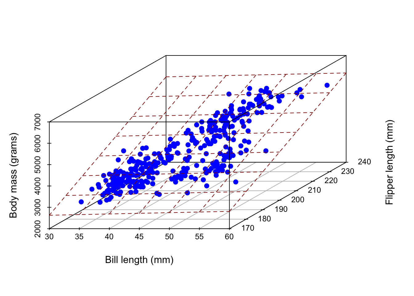
Example: many numerical predictors
bm_fl_bl_fit <- linear_reg() |>
  fit(body_mass_g ~ flipper_length_mm + bill_length_mm, data = penguins)

tidy(bm_fl_bl_fit)
# A tibble: 3 × 5
term estimate std.error statistic p.value
<chr> <dbl> <dbl> <dbl> <dbl>
1 (Intercept) -5737. 308. -18.6 7.80e-54
2 flipper_length_mm 48.1 2.01 23.9 7.56e-75
3 bill_length_mm 6.05 5.18 1.17 2.44e- 1\[ \small\widehat{body~mass}=-5736+48.1\times flipper~length+6\times bill~length \]
Example: many numerical predictors
Welcome to statistics!
The code was basically the same every time. In this part of the course, the code itself is not the primary complication. The code is merely a labor-saving device. Our focus shifts to understanding the conceptual and technical underpinnings of the code and interpreting the output correctly. This is subtle, and it tends to trip people up.
FAQ
Does it matter what the base level is?
Regarding the leveling of a categorical predictor:
- It doesn’t matter technically. The math doesn’t care;
- As long as you know what the baseline is, you are consistent throughout your analysis, and you interpret everything correctly, you’re probably good;
- Sometimes the application suggests a natural choice of baseline. You make interpretation and visualization easier if you respect that.
Is interaction the same as separate regressions?
Sort of. You get the same estimates of the slopes and intercepts, but the uncertainty quantification (standard errors) is different.
The interaction model
linear_reg() |>
  fit(body_mass_g ~ flipper_length_mm * island, data = penguins) |>
  tidy() |>
  select(term, estimate, std.error)
# A tibble: 6 × 3
term estimate std.error
<chr> <dbl> <dbl>
1 (Intercept) -5464. 431.
2 flipper_length_mm 48.5 2.05
3 islandDream 3551. 969.
4 islandTorgersen 3218. 1680.
5 flipper_length_mm:islandDream -19.4 4.94
6 flipper_length_mm:islandTorgersen -17.4 8.73So on Biscoe island (where Dream = Torgersen = 0), the line is
\[ \begin{aligned} \widehat{body~mass} = -5464 &+ 48.5 \times flipper~length \end{aligned} \]
Simple regression within a group
If we fit a simple model with the Biscoe subset of the data:
penguins_biscoe <- penguins |>
  filter(island == "Biscoe")

linear_reg() |>
  fit(body_mass_g ~ flipper_length_mm, data = penguins_biscoe) |>
  tidy()
# A tibble: 2 × 5
term estimate std.error statistic p.value
<chr> <dbl> <dbl> <dbl> <dbl>
1 (Intercept) -5464. 435. -12.6 8.48e-26
2 flipper_length_mm 48.5 2.07 23.4 2.20e-54Same estimates, but different standard errors.
The default picture
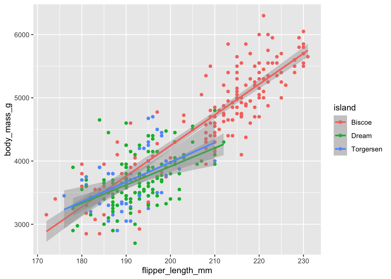
These are separate simple regressions within each group. The slopes and the intercepts are the same as the interaction model, but the uncertainty bands are different.
A second look at \(R^2\)
Recap: our first look
\(R^2\) measures “goodness-of-fit:”
- \(R^2\) is “a Rotten Tomatoes score” for your model;
- It ranges from 0 (horrific) to 1 (perfect) and measures how well the linear model fits the data;
- In simple linear regression with one numerical predictor, \(R^2\) is literally equal to the square of the correlation coefficient between the predictor \(X\) and the numerical response \(Y\);
- When you move from one predictor to many, this relationship breaks down, but \(R^2\) remains meaningful.
So what is it, actually?
What is “goodness-of-fit”?
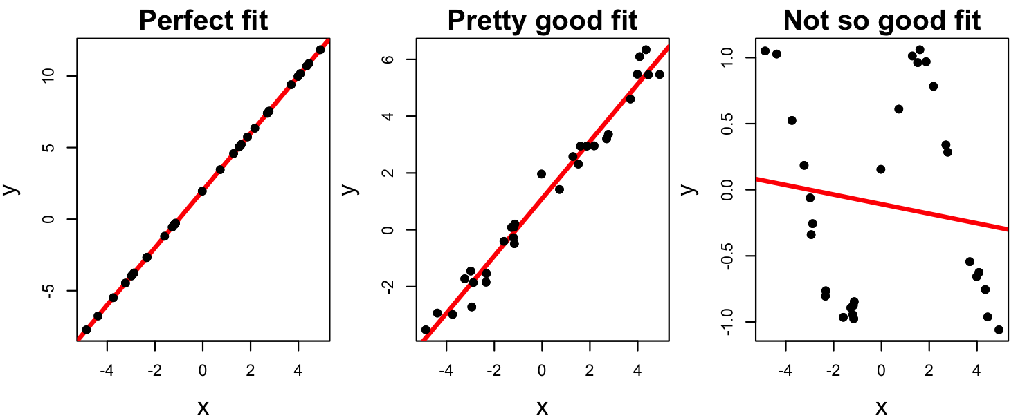
- Quality of fit appears to have something to do with how “all over the place” the residuals are;
- We want to quantify this intuition with a concrete numerical measure that we can use to rank competing models according to goodness-of-fit.
Reminder: residuals
Every data point has one:
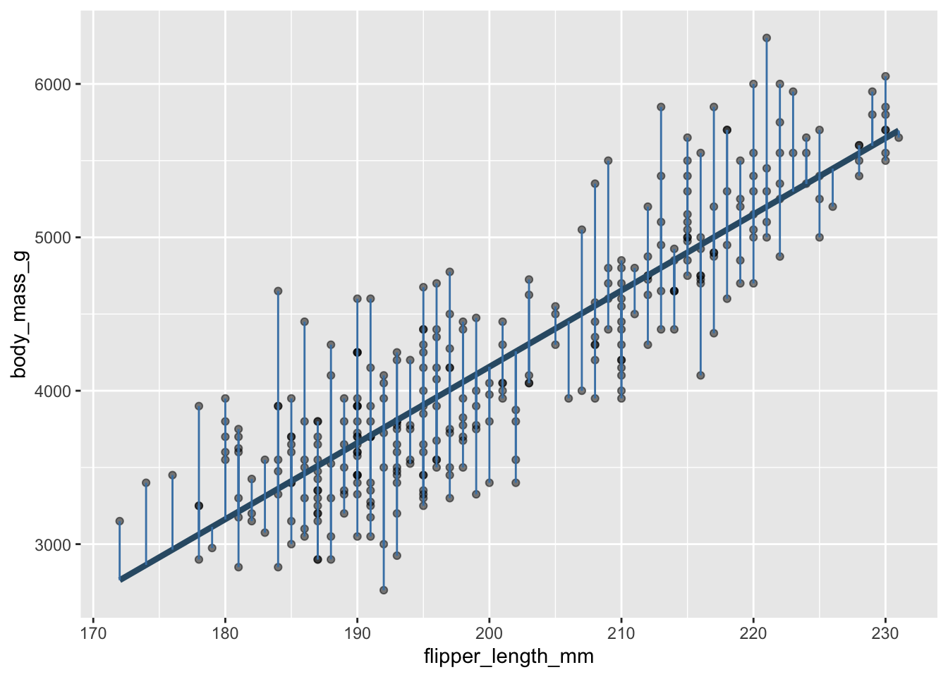
Some are big, some are small. Some are above the line (positive), and some are below the line (negative).
Reminder: residuals
The residuals are what’s “left over” after the model attempts to “explain” the response:
\[ e_i = \text{observed} - \text{predicted} = y_i - \hat{y}_i. \]
Every data point has one:
# A tibble: 344 × 4
   flipper_length_mm body_mass_g .pred  .resid
               <int>       <int> <dbl>   <dbl>
 1               181        3750 3212.  538.
 2               186        3800 3461.  339.
 3               195        3250 3908. -658.
 4                NA          NA   NA    NA
 5               193        3450 3808. -358.
 6               190        3650 3659.   -9.43
 7               181        3625 3212.  413.
 8               195        4675 3908.  767.
 9               193        3475 3808. -333.
10               190        4250 3659.  591.
# ℹ 334 more rows
how it started vs. how it's going
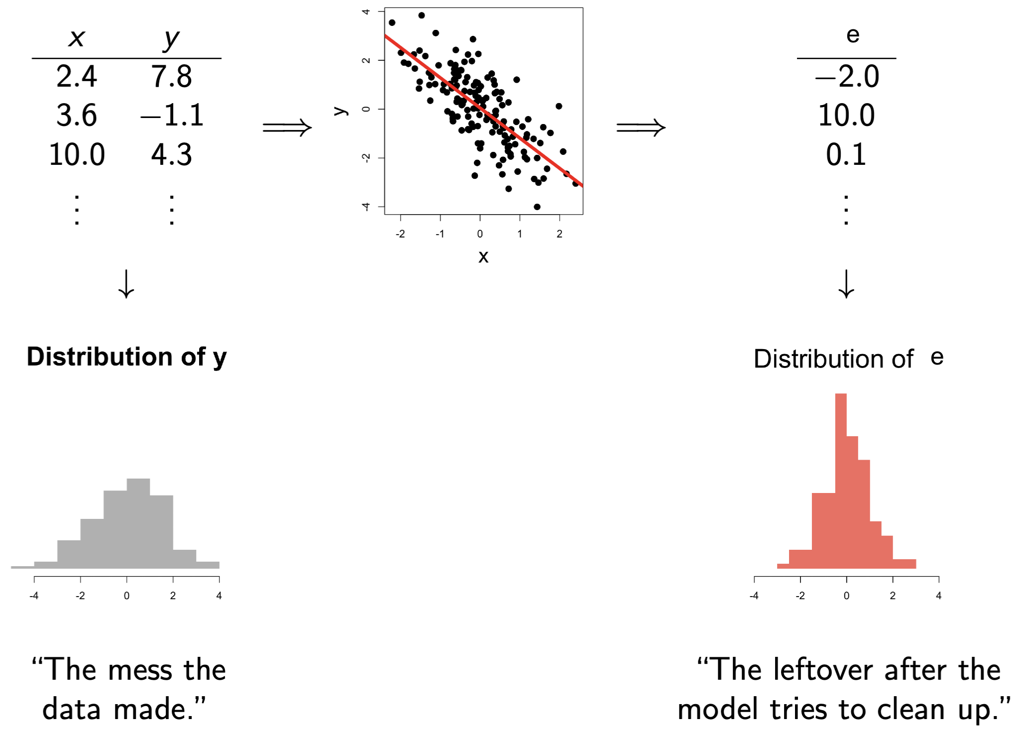
How it started
The original distribution of the response. This is the mess we’re trying to clean up with a model:
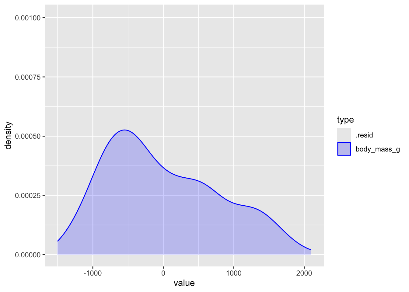
# A tibble: 1 × 3
  type        variance   std
  <chr>          <dbl> <dbl>
1 body_mass_g  643131.  802.
How it’s going
The distribution of the residuals (the leftover mess) after the model tries to explain (clean up):
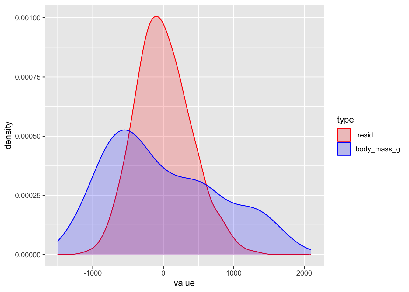
# A tibble: 2 × 3
  type        variance   std
  <chr>          <dbl> <dbl>
1 .resid       154999.  394.
2 body_mass_g  643131.  802.
The main idea
The model is trying to “explain” the variation in the response:
- Variation in the response (blue distribution), is the mess we’re trying to clean up;
- Variation in the residuals (red distribution), is the leftover after the model gives it a shot;
- The more leftover there is, the worse the model did;
- You can quantify this with the variance. The smaller the variance of the residuals relative to the original response variance, the better.
That’s what \(R^2\) actually is: the proportion of the variance in the response explained by the model.
\(R^2\approx 0\)
Horrifically awful fit. The model didn’t explain (clean up) anything:
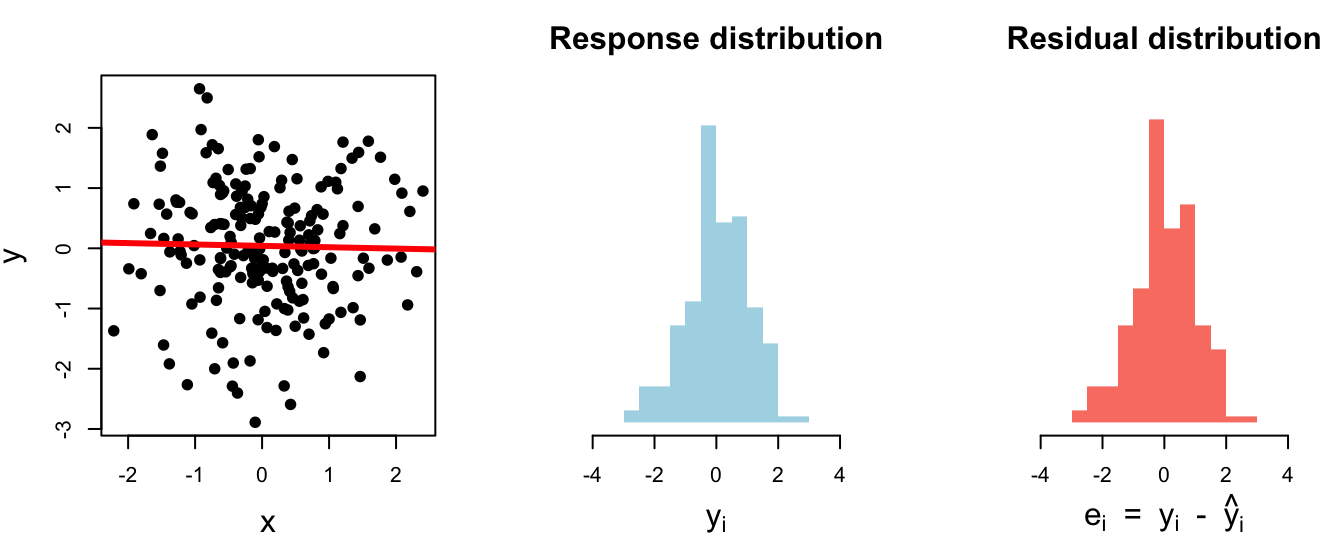
# A tibble: 1 × 3
  var_y var_resid r.squared
  <dbl>     <dbl>     <dbl>
1  1.02      1.02  0.000450
\(R^2\approx 0.28\)
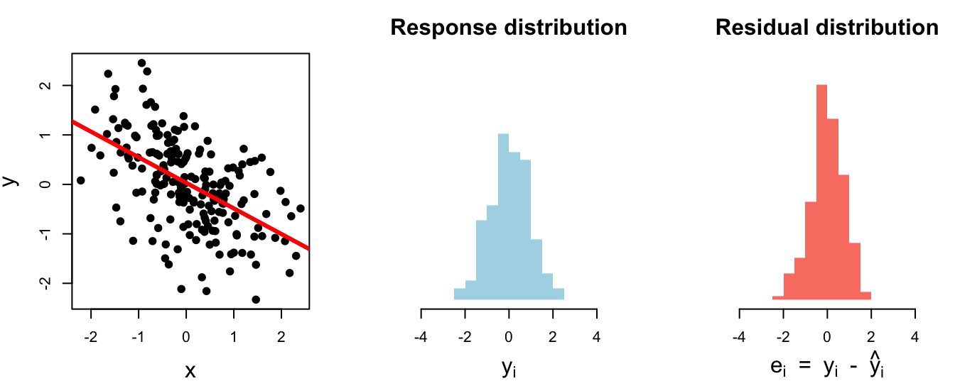
# A tibble: 1 × 3
  var_y var_resid r.squared
  <dbl>     <dbl>     <dbl>
1 0.805     0.574     0.287
\(R^2\approx 0.63\)
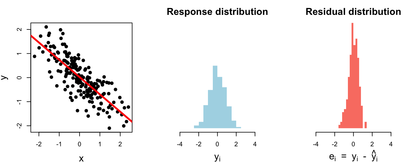
# A tibble: 1 × 3
  var_y var_resid r.squared
  <dbl>     <dbl>     <dbl>
1 0.701     0.255     0.636
\(R^2\approx 0.97\)
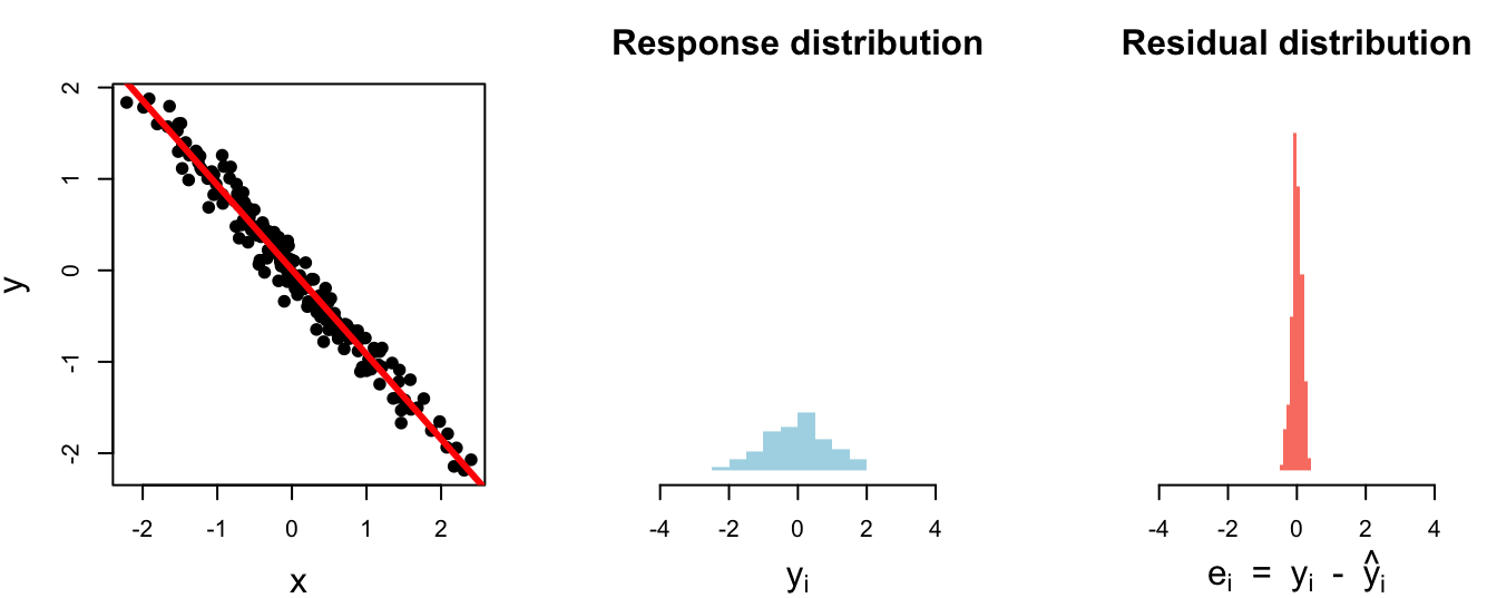
# A tibble: 1 × 3
  var_y var_resid r.squared
  <dbl>     <dbl>     <dbl>
1 0.762    0.0230     0.970
\(R^2\approx 1\)
Perfect fit. The model explained (cleaned up) everything:
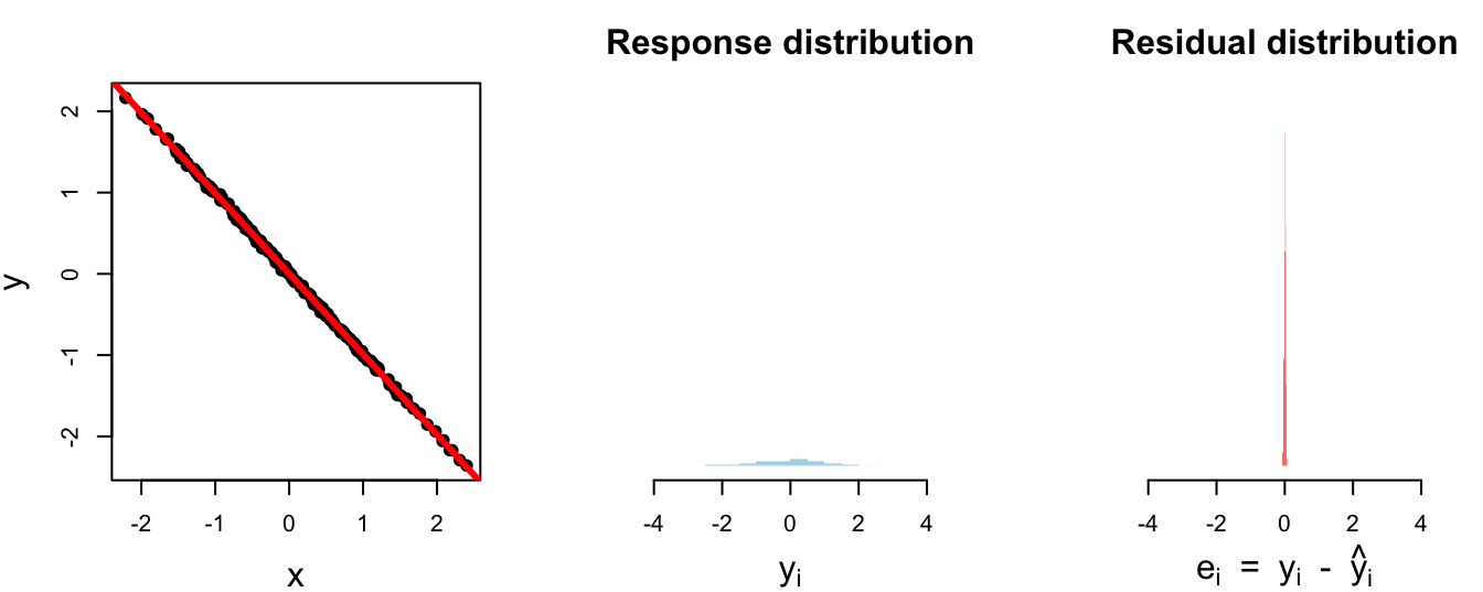
# A tibble: 1 × 3
  var_y var_resid r.squared
  <dbl>     <dbl>     <dbl>
1 0.847  0.000408     1.000
The nitty gritty
\[ \begin{aligned} R^2\, &= \begin{matrix} \text{proportion of}\\ \text{variation explained} \end{matrix} \\[15pt] &= 1- \begin{matrix} \text{proportion of}\\ \text{variation unexplained} \end{matrix}\\[15pt] &= 1-\frac{\text{unexplained variation}}{\text{total variation}} \\[15pt] &= 1-\frac{\texttt{how it's going}}{\texttt{how it started}} \\[15pt] &= 1-\frac{\text{spread of leftover}}{\text{spread of original mess}} \\[15pt] &= 1-\frac{\text{spread of residuals}}{\text{spread of response}} \\[15pt] &= 1-\frac{\text{var}(e_i)}{\text{var}(y_i)} . \end{aligned} \]
Literally
Basic facts
- We always have \(\text{var}(y_i)\geq \text{var}(e_i)\), so \(0\leq R^2\leq 1\);
- If \(\text{var}(e_i)=0\), then the model explained everything, the fit is perfect (poifect!), and
\[ R^2=1-\frac{\text{var}(e_i)}{\text{var}(y_i)}=1-\frac{0}{\text{var}(y_i)}=1-0=1. \]
- If \(\text{var}(e_i)=\text{var}(y_i)\), then the model explained nothing, the fit is perfectly wretched, and
\[ R^2=1-\frac{\text{var}(e_i)}{\text{var}(y_i)}=1-\frac{\text{var}(y_i)}{\text{var}(y_i)}=1-1=0. \]
Summary
\(R^2\) is a number between zero and one, and it represents the proportion of the variance in the response \(Y\) that is explained by the model fit;
This is the interpretation, regardless how many predictors you have;
In simple regression with one numerical predictor, \(R^2\) it is also the square of the correlation coefficient, but this doesn’t generalize to the multivariate setting.
Model selection
Model selection
Question: Given many competing models for the same response, which model is “best”? What does that even mean?
Answer: Assign a “quality score” to each model, and pick the model with the best score:
| Model | Score | Verdict |
|---|---|---|
| Simple | 0.1 | ❌ |
| Additive | 0.5 | ✅ |
| Interaction | 0.48 | ❌ |
Variable selection: all of our models were linear, and they differed only by which predictor variables are included. By ranking models by quality score and picking the “best” one, we can determine which predictors are the “most important” to include.
Selection criteria
This is a big area of statistical research. There are loads of “quality scores” you could consider, and they prioritize different things: predictive accuracy, goodness-of-fit, simplicity, fairness, etc.
- \(R^2\)
- adjusted \(R^2\)
- Akaike Information criterion (AIC)
- Bayesian information criterion (BIC)
- … so many more
We won’t go into detail, but you will if you keep studying statistics.
tidymodels reports many of these for free
\(R^2\)’s dirty little secret
\(R^2\) gives participation trophies. It always goes up when you add any new variable to the model, even if that variable is worthless.
Adding a phony variable
The original model fit:
[1] 0.7589925Adjusted \(R^2\)
Because vanilla \(R^2\) blithely rewards the addition of any variable, no matter how meaningless, you shouldn’t use it for model selection. Instead, use adjusted \(R^2\). The formula is in the textbook if you’re dying to know, but here’s the tea:
- adjusted \(R^2\) penalizes the inclusion of unnecessary predictors;
- It prioritizes a parsimonious model:
- a model that fits/predicts well, and…
- a model that’s not too complicated (so our pea brains can still understand it);
- Occam’s razor!
For the penguins
Balancing fit and complexity
More complex models (i.e., models with more predictors) tend to fit the data at hand better, but may not generalize well to new data.
Model selection criteria, like adjusted \(R^2\), help balance model fit and complexity to avoid overfitting by penalizing models with more predictors.
Overfitting
Overfitting occurs when a model captures not only the underlying relationship between predictors and outcome but also the random noise in the data.
-
Overfitted models tend to perform well on the observed data but poorly on new, unseen data.
- Good news: We have techniques to detect and prevent overfitting.
- Bad news: We won’t get into those until next week.
Back to variable selection
Given a set of competing models, all trying to predict the same response, we can line ’em up, compute adjusted \(R^2\) for each model, and then pick the model with the highest score.
Easy, right?

Listing out all the possible models
- The penguins dataset has \(p=6\) variables apart from body mass: species, island, bill length, bill depth, flipper length, and sex;
- How many models is that (ignoring the possibility of interaction, which makes things worse):
- 1 “empty” model: include no predictors;
- 6 “simple” models: include only one predictor;
- 15 two-predictor models;
- 20 three-predictor models;
- 15 four-predictor models;
- 6 five-predictor models;
- 1 “full” model: include all predictors.
- That’s \(2^6=64\) models in total you have to consider. Not the end of the world if you have a computer, but it gets worse…
Combinatorial explosion
- If you have \(p\) candidate predictors, then the set of all possible subsets you could include in a model grows very quickly;
- In the “big data” era, 100 predictors is amateur hour, so it becomes infeasible to fit every possible model;
- It pays to “search” through the space of models in a smarter, less brute-force way.
| \(p\) | # of models = \(2^p\) |
|---|---|
| 2 | 4 |
| 5 | 32 |
| 10 | 1024 |
| 20 | 1048576 |
| 30 | 1073741824 |
| 40 | \(\approx 1.098\times 10^{12}\) |
| 50 | \(\approx 1.13\times 10^{15}\) |
| 100 | \(\approx 1.27\times 10^{30}\) |
Backward elimination
Start with the full model (the model that includes all potential predictor variables). Variables are eliminated one-at-a-time from the model until we cannot improve the model any further.
Procedure:
- Start with a model that has all predictors we consider and compute the adjusted \(R^2\).
- Next fit every possible model with 1 fewer predictor.
- Compare adjusted \(R^2\)s to select the best model (highest adjusted \(R^2\)) with 1 fewer predictor.
- Repeat steps 2 and 3 until adjusted \(R^2\) no longer increases.
Foreward stepwise regression
Forward stepwise regression is the reverse of the backward elimination technique. Instead, of eliminating variables one-at-a-time, we start from an “empty model” and we add variables one-at-a-time until we cannot find any variables that improve the model any further.
Procedure:
- Start with a model that has no predictors.
- Next fit every possible model with 1 additional predictor and calculate adjusted \(R^2\) of each model.
- Compare adjusted \(R^2\) values to select the best model (highest adjusted \(R^2\)) with 1 additional predictor.
- Repeat steps 2 and 3 until adjusted \(R^2\) no longer increases.