Linear models with a single predictor

Lecture 5

John Zito

Duke University
STA 101 Fall 2026

2026-09-15

Correlation vs. causation

Spurious correlations

Source: tylervigen.com/spurious-correlations

Spurious correlations

Source: tylervigen.com/spurious-correlations

Watch out!

• On its own, a linear regression model can only summarize association (eg. correlation) among variables. Whether or not it has anything to say about causation is a delicate matter, one that we will confront head-on after fall break;
• For now, think like we’re still just doing exploratory analysis: visualizing and summarizing.

Simple Linear Regression

Data prep

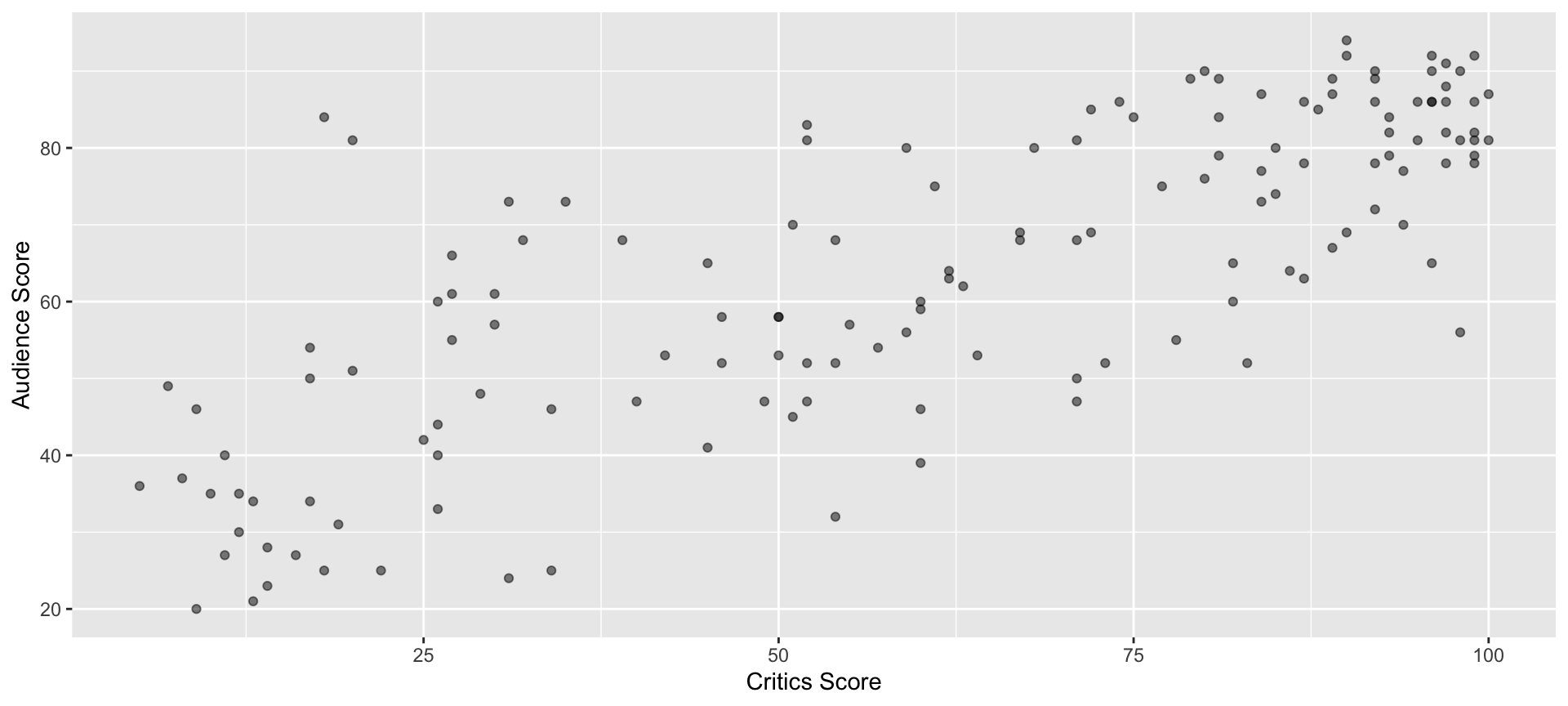
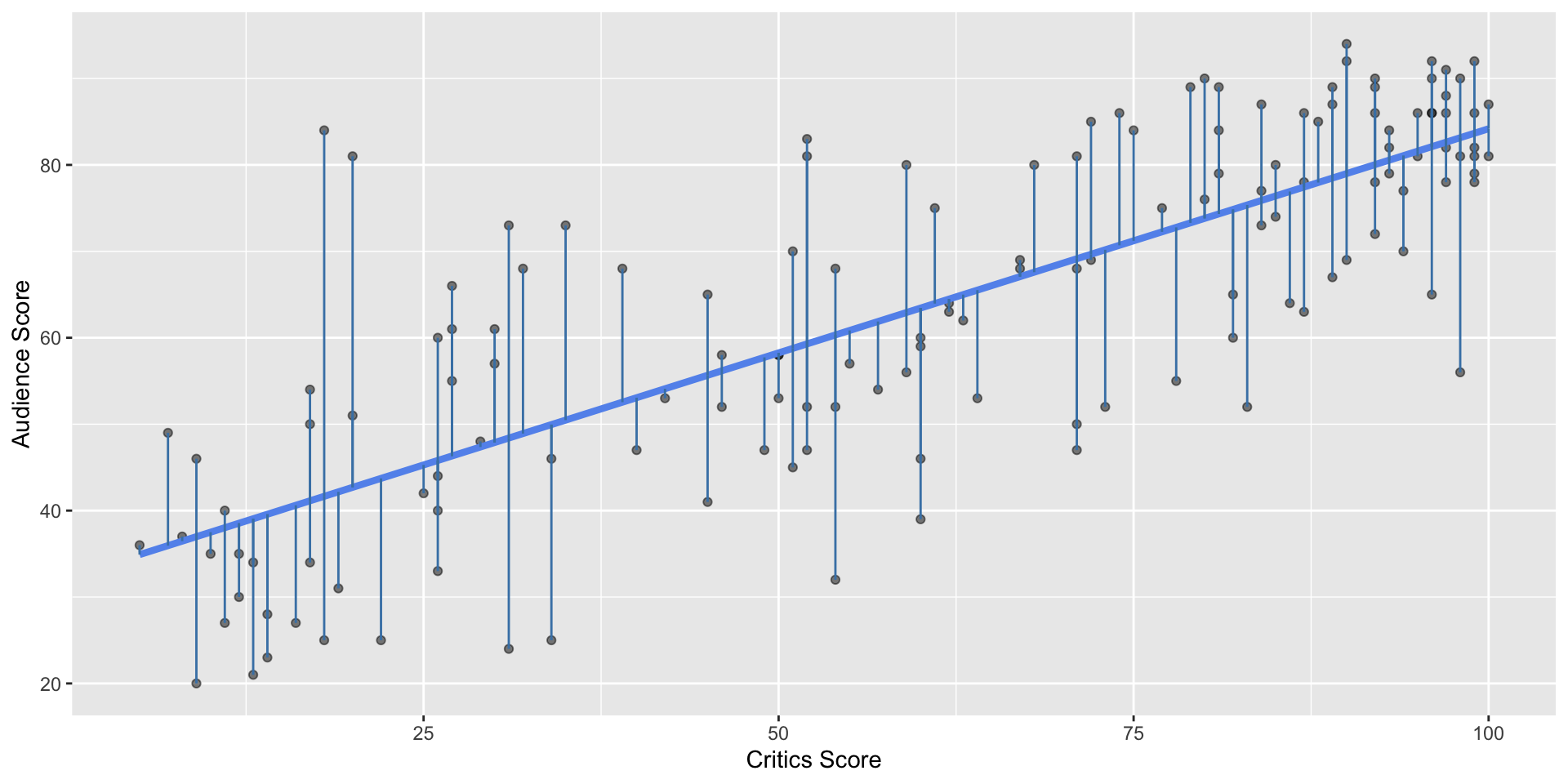
• Rename Rotten Tomatoes columns as critics and audience
• Rename the dataset as movie_scores

movie_scores <- fandango |>
  rename(
    critics = rottentomatoes, 
    audience = rottentomatoes_user
  )

Data overview

movie_scores |>
  select(critics, audience)

# A tibble: 146 × 2
   critics audience
     <int>    <int>
 1      74       86
 2      85       80
 3      80       90
 4      18       84
 5      14       28
 6      63       62
 7      42       53
 8      86       64
 9      99       82
10      89       87
# ℹ 136 more rows

Data visualization

Quick aside: which is which?

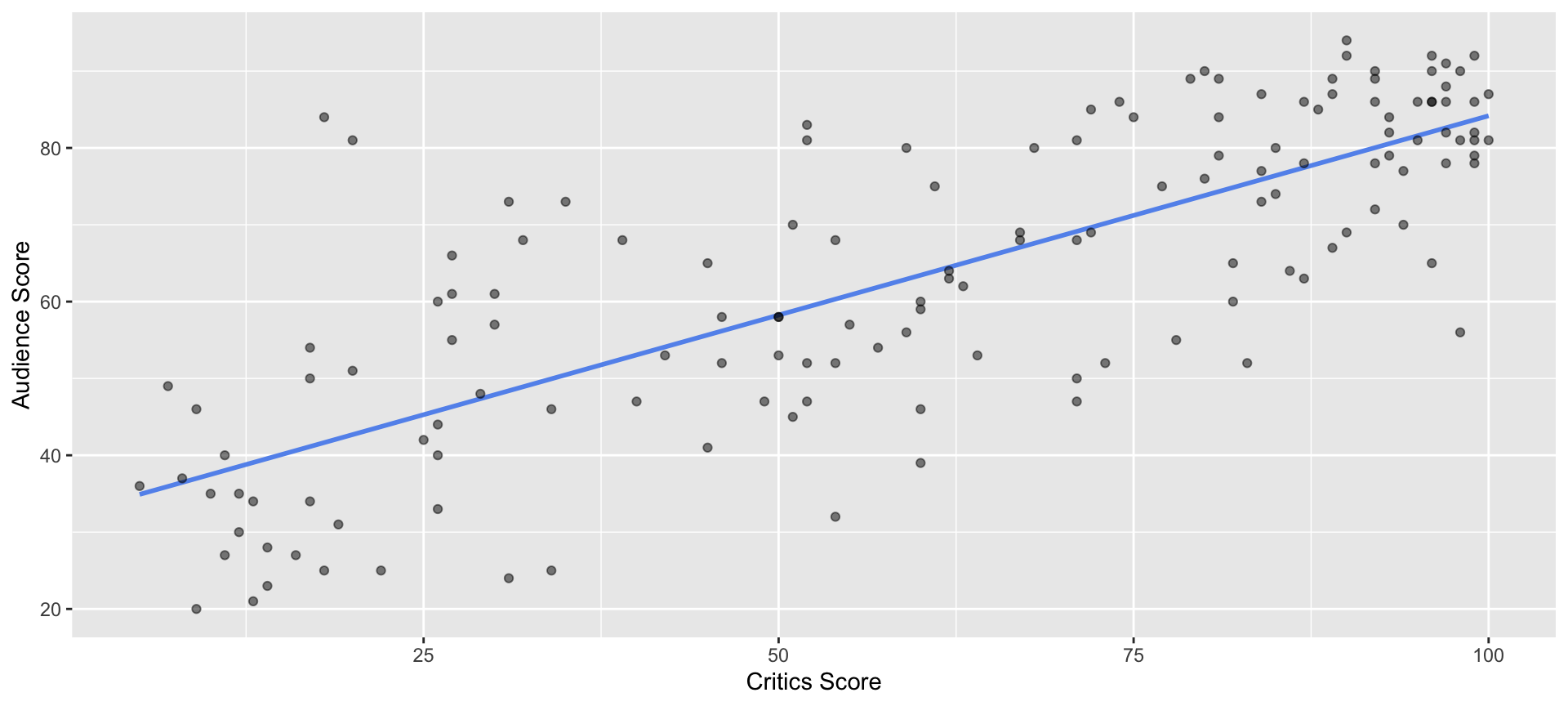
How do we know which variable “should” be the response and which should be the predictor. This will depend on the domain and the research question, but in some cases there is a natural choice. In this example, the critic score for a film is typically available before the audience score. Critics can often screen the film in advance, and their reviews are published on opening day. By contrast, the audience score trickles in over the subsequent weeks. So it’s more likely that we would already have the critics score and use it to anticipate the audience score, instead of the other way around.

Similar story to our other examples:

• budget versus revenue of films;
• weight versus MPG of cars;
• temperature versus ice duration of lakes.

Which variable is available first, or easier to measure? In which direction would we typically be predicting?

Data visualization: linear model

# A tibble: 2 × 5
  term        estimate std.error statistic  p.value
  <chr>          <dbl>     <dbl>     <dbl>    <dbl>
1 (Intercept)   32.3      2.34        13.8 4.03e-28
2 critics        0.519    0.0345      15.0 2.70e-31

# A tibble: 1 × 1
      r
  <dbl>
1 0.781

Prediction

new_movies <- tibble(
  critics = c(20, 37.5, 88)
)

predict(audience_critic_fit, 
        new_data = new_movies)

# A tibble: 3 × 1
  .pred
  <dbl>
1  42.7
2  51.8
3  78.0

augment(audience_critic_fit,
        new_data = new_movies)

# A tibble: 3 × 2
  .pred critics
  <dbl>   <dbl>
1  42.7    20  
2  51.8    37.5
3  78.0    88  

What is this line and how was it drawn?

Regression model

A regression model is a function that describes the relationship between the outcome \(Y\) and the predictor \(X\).

\[ \begin{aligned} Y &= \color{black}{\textbf{Model}} + \text{Error} \\[8pt] &= \color{black}{\mathbf{f(X)}} + \epsilon \\[8pt] &= \color{black}{\boldsymbol{\mu_{Y|X}}} + \epsilon \end{aligned} \]

\(\mu_{Y \mid X}\) is the expected value of \(Y\) given (“conditional on”) a particular value of \(X\).

Regression model

\[ \begin{aligned} Y &= \color{#6495ED}{\textbf{Model}} + \text{Error} \\[8pt] &= \color{#6495ED}{\mathbf{f(X)}} + \epsilon \\[8pt] &= \color{#6495ED}{\boldsymbol{\mu_{Y|X}}} + \epsilon \end{aligned} \]

Simple linear regression

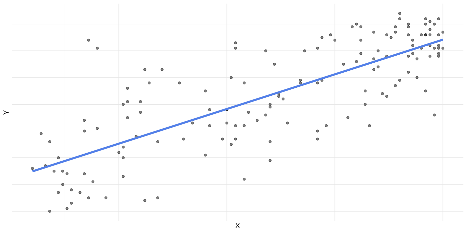
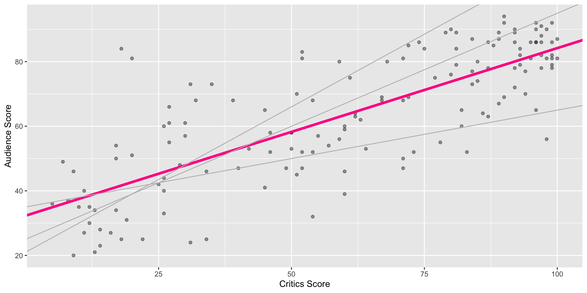
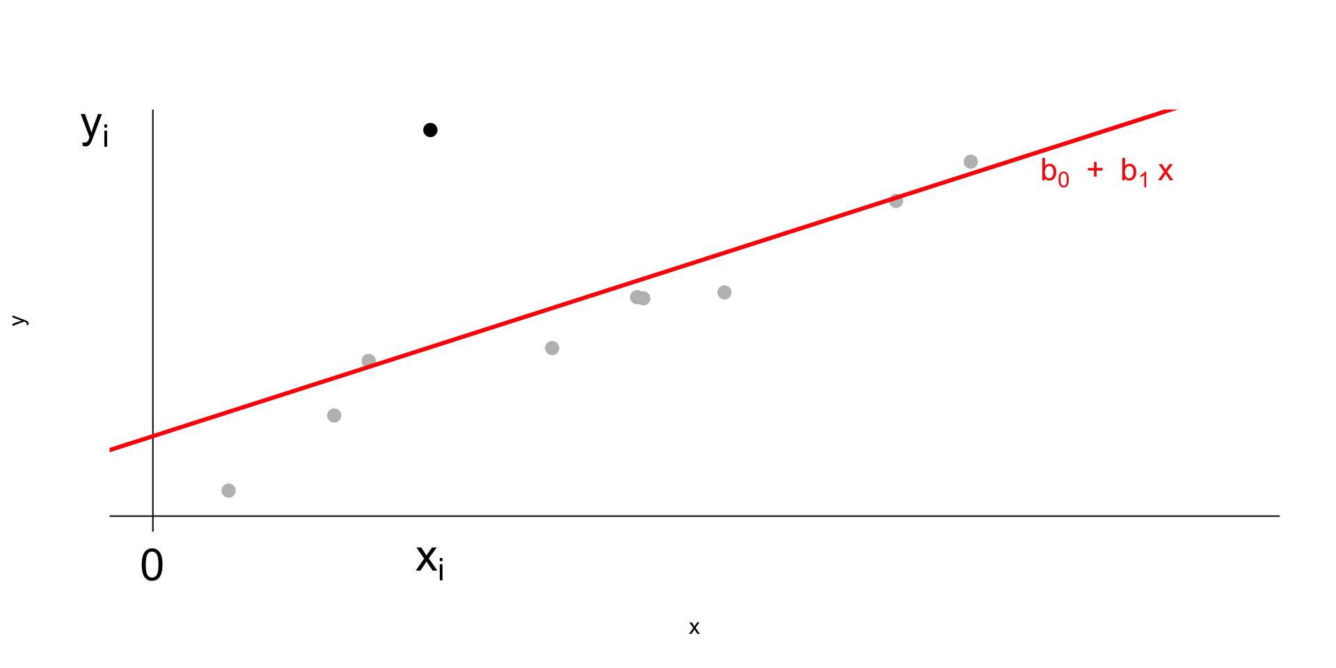
• Use simple linear regression to model the relationship between a quantitative outcome (\(Y\)) and a single quantitative predictor (\(X\))

• The “idealized” linear regression model, revealed only with infinite data:

\[\Large{Y = \beta_0 + \beta_1 X + \epsilon}\]

• \(\beta_1\): True slope of the relationship between \(X\) and \(Y\)
• \(\beta_0\): True intercept of the relationship between \(X\) and \(Y\)
• \(\epsilon\): Error (residual)

Simple linear regression

• The “fitted” model, obtained by estimating \(\beta_0\) and \(\beta_1\) using a finite sample (\(x_1, y_1\)), (\(x_2, y_2\)), …, (\(x_n, y_n\))

\[\Large{\widehat{Y} = b_0 + b_1 X}\]

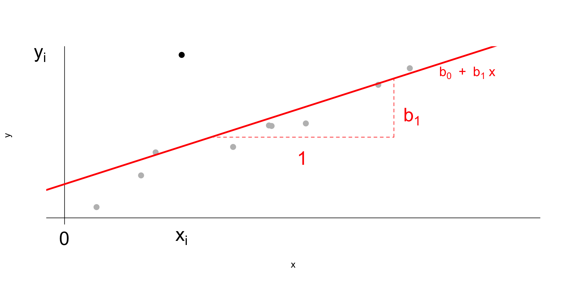
• \(b_1\): Estimated slope of the relationship between \(X\) and \(Y\); you may also see \(\widehat{\beta_1}\)

• \(b_0\): Estimated intercept of the relationship between \(X\) and \(Y\); you may also see \(\widehat{\beta_0}\)

• No error term!

• Ideally, as \(n \to \infty\), \(b_0 \to \beta_0\) and \(b_1 \to \beta_1\)

Why did the notation change?

You’re already familiar with \(y=mx+b\), so why did I switch it up on you? Why the subscripts? Why the Greek letters?

• Today, we’re studying simple linear regression where there is only one predictor. Soon, we will study multiple linear regression, where there are >1 predictors, and each one gets its own coefficient. When you go from 1 predictor to 5 or 10 or 1,000, you run out of letters. So it’s easier to add subscripts to the same letter;
• The Greek letters denote true, idealized, population values. These are unknown. If we had perfect data, we would know them, but we don’t;
• The lowercase roman letters denote estimated values based on a finite, imperfect sample. These are our best guess at the true values based on the data we have.

Choosing values for \(b_1\) and \(b_0\)

Residuals

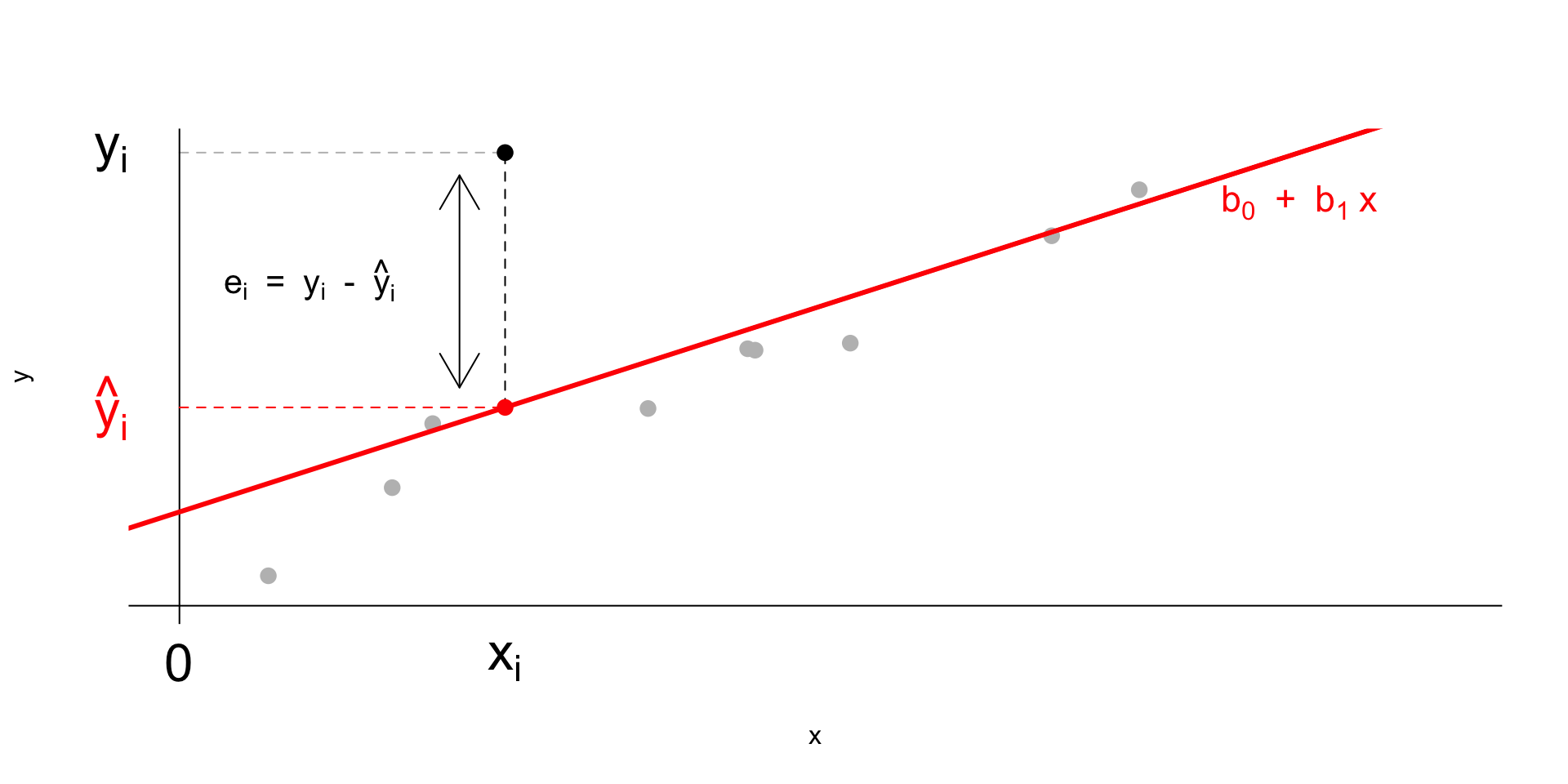
\[\text{residual} = \text{observed} - \text{predicted} = y - \widehat{y}\]

Notation

• We have \(n\) observations (generally, the number of rows in a df)

• \(i^{th}\) observation (\(i\) from \(1\) to \(n\)):

  • \(y_i\) : \(i^{th}\) outcome

  • \(x_i\) : \(i^{th}\) explanatory variable

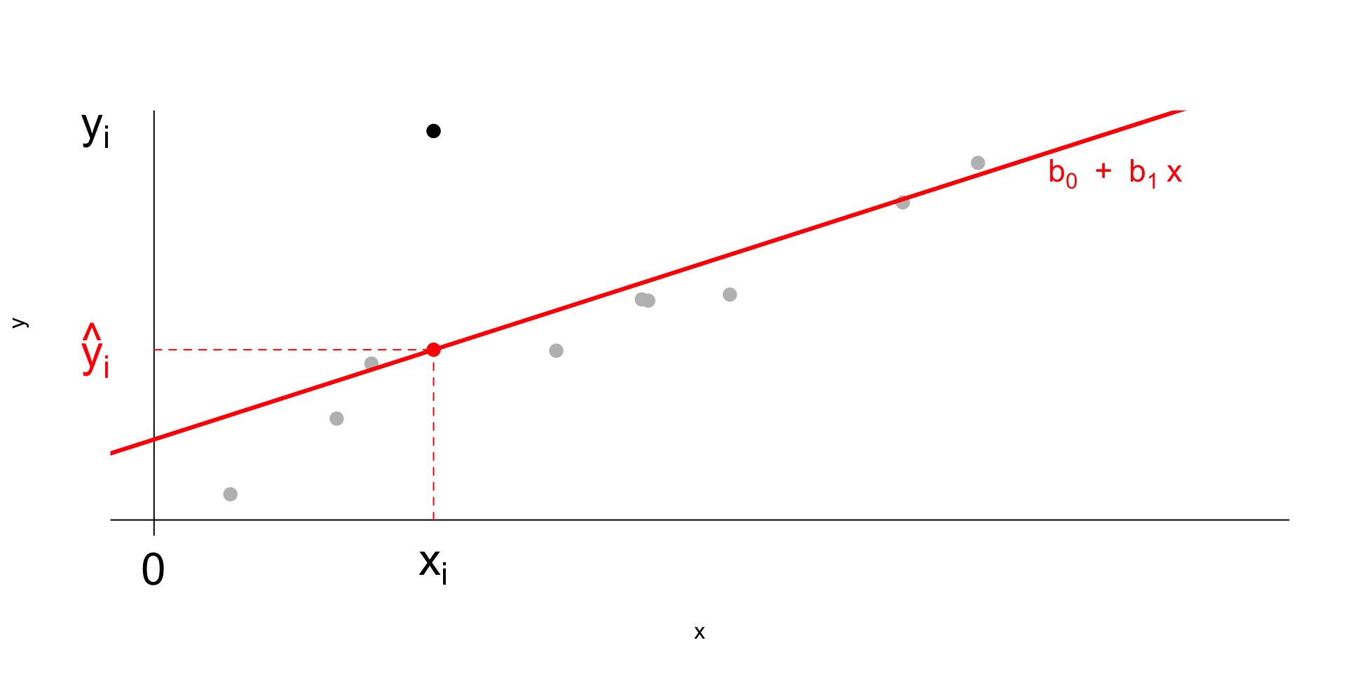
  • \(\widehat{y_i}\) : \(i^{th}\) predicted outcome

  • \(e_i\) : \(i^{th}\) residual

Least squares line

• The residual for the \(i^{th}\) observation is

\[e_i = \text{observed} - \text{predicted} = y_i - \widehat{y}_i\]

• The sum of squared residuals is

\[e^2_1 + e^2_2 + \dots + e^2_n\]

• The least squares line is the one that minimizes the sum of squared residuals (SSR)

Perhaps more clearly…

data		residuals
\(x_1 \quad y_1\)	\(\rightarrow\)	\(e_1 = y_1 - \widehat{y_1} = y_1 - (b_0 + b_1 \times x_1)\)
\(x_2 \quad y_2\)	\(\rightarrow\)	\(e_2 = y_2 - \widehat{y_2} = y_2 - (b_0 + b_1 \times x_2)\)
\(x_3 \quad y_3\)	\(\rightarrow\)	\(e_3 = y_3 - \widehat{y_3} = y_3 - (b_0 + b_1 \times x_3)\)
…	\(\rightarrow\)	…
\(x_n \quad y_n\)	\(\rightarrow\)	\(e_n = y_n - \widehat{y_n} = y_n - (b_0 + b_1 \times x_n)\)

\[ \downarrow \]

\[ e_1^2 + e_2^2 + e_3^2 + \ldots + e_n^2 \]

sum of squared residuals

We pick \(b_0\) and \(b_1\) so that

\[ \sum_{i=1}^{n} e_i^2 \]

is as small as possible (“best fit”).

Why “least-squares” regression?

Why do we minimize

\[ \sum_{i=1}^{n} e_i^2, \]

and not

\[ \sum_{i=1}^{n} e_i, \]

or

\[ \sum_{i=1}^{n} |e_i| \; ? \]

Why not minimize \(\sum e_i\)?

Suppose our residuals are

\[ -4,\; -2,\; 1,\; 2,\; 3 \]

Then

\[ \sum_{i=1}^n e_i = (-4)+(-2)+1+2+3 = 0. \]

But the predictions are clearly not perfect!

Problem: Positive and negative residuals cancel each other out.

\[ -4 + 4 = 0 \]

even though both residuals represent prediction errors.

Why squared errors help

Using the same residuals,

\[ -4,\; -2,\; 1,\; 2,\; 3 \]

the sum of squared residuals is

\[ (-4)^2 + (-2)^2 + 1^2 + 2^2 + 3^2 = 34. \]

Now all prediction errors contribute positively to the summation.

• Large errors count more heavily (i.e., we are penalizing larger residuals);
• Positive and negative errors cannot cancel;
• The “best” line has the smallest total squared error.

Why not just minimize \(\sum |e_i|\)?

Absolute error solves the cancellation problem:

\[ -4,\; -2,\; 1,\; 2,\; 3 \]

\[ |{-4}| + |{-2}| + |1| + |2| + |3| = 12 \]

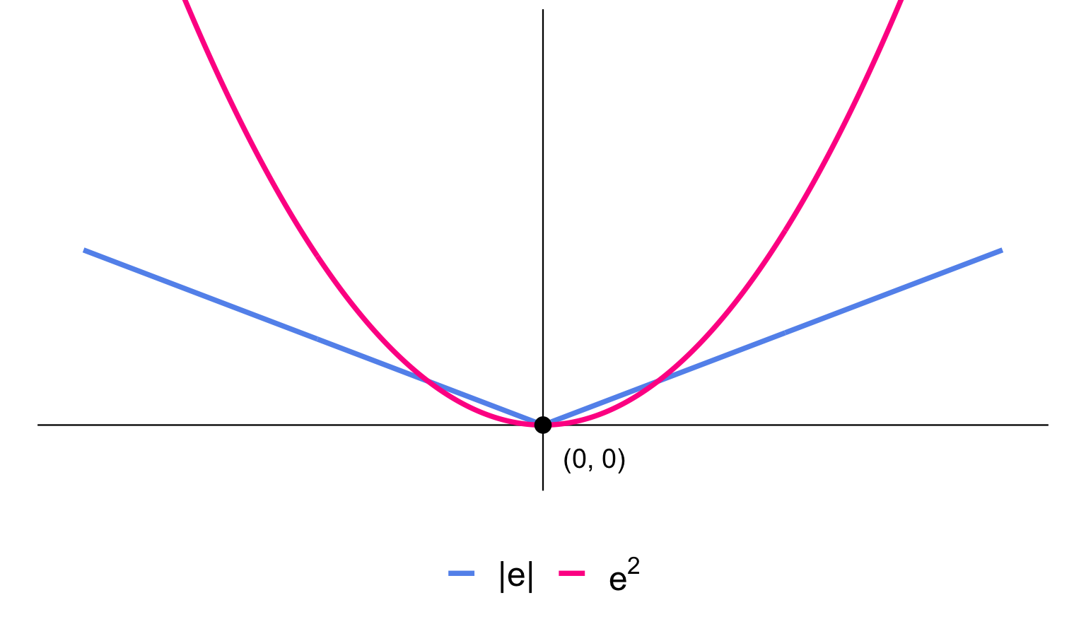
So every prediction error contributes positively. However, squared error has an important advantage:

\[ e^2 \]

is a smooth curve, while

\[ |e| \]

has a sharp point at \(e=0\).

As a result:

• Squared error is easier to optimize mathematically (derivative exists for all points);
• Squared error leads to a simple formula for the regression line;
• Large mistakes are penalized more heavily.

Therefore, we usually minimize

\[ \sum_{i=1}^n e_i^2. \]

Put in a picture…

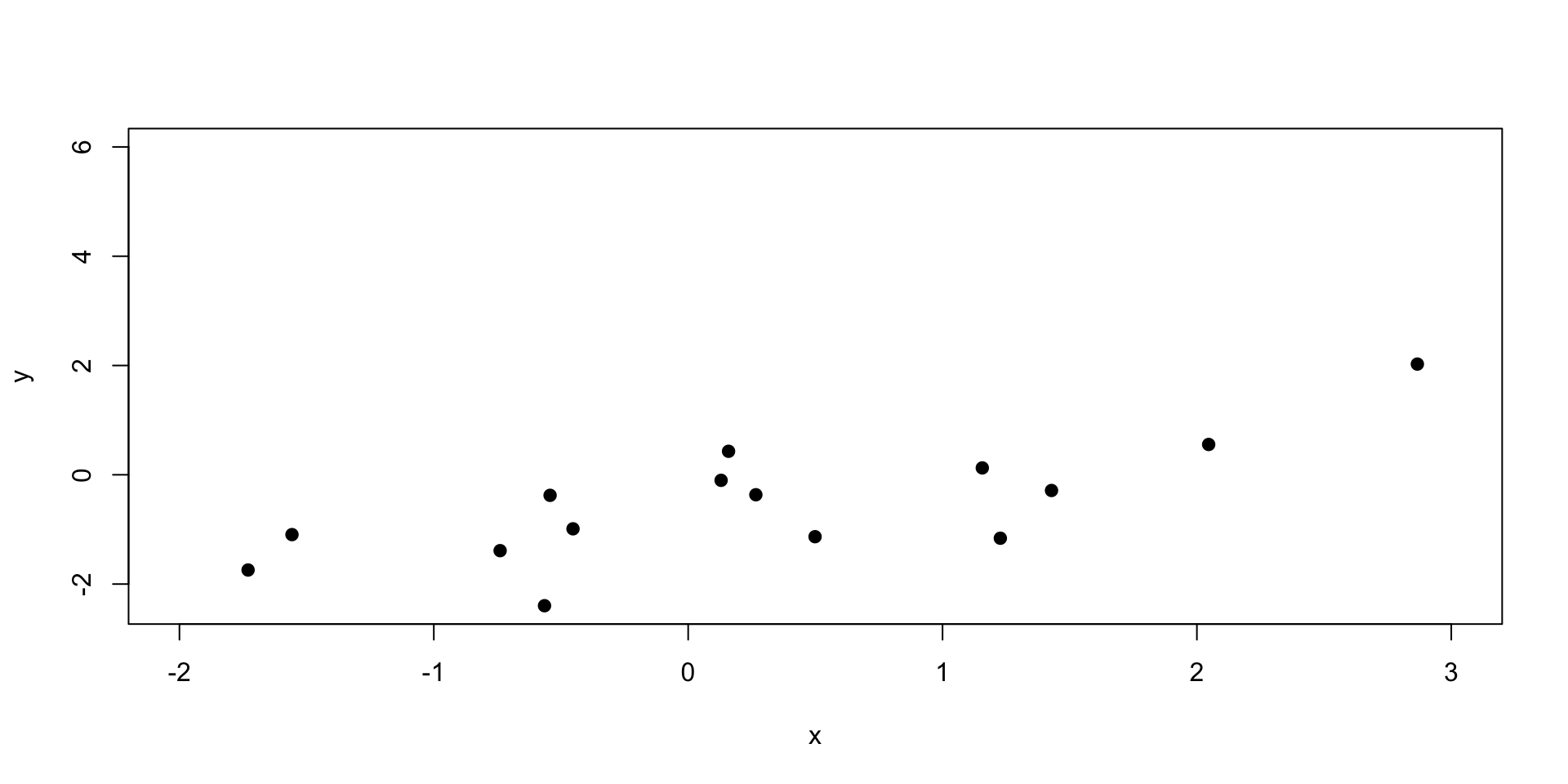
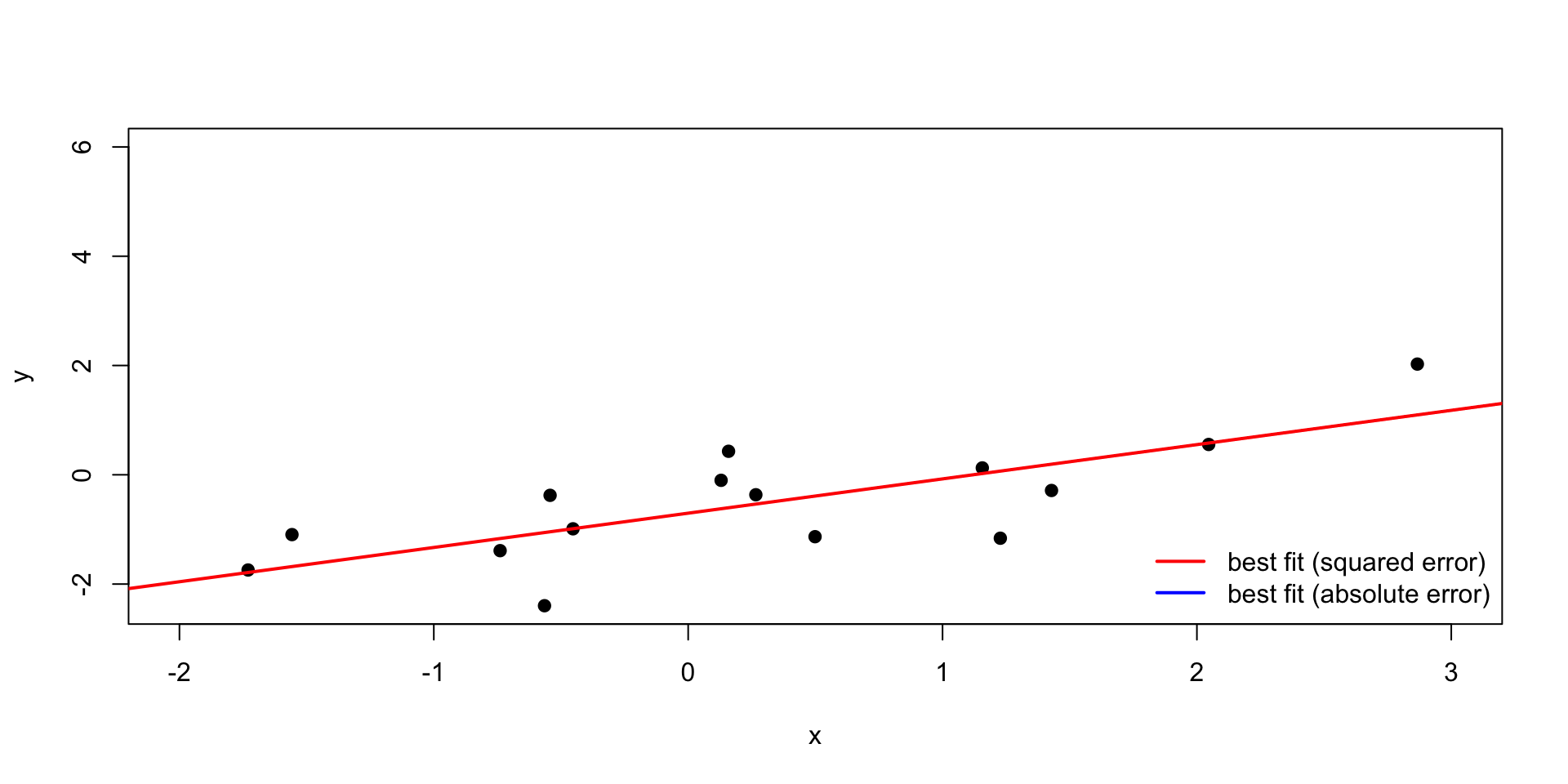
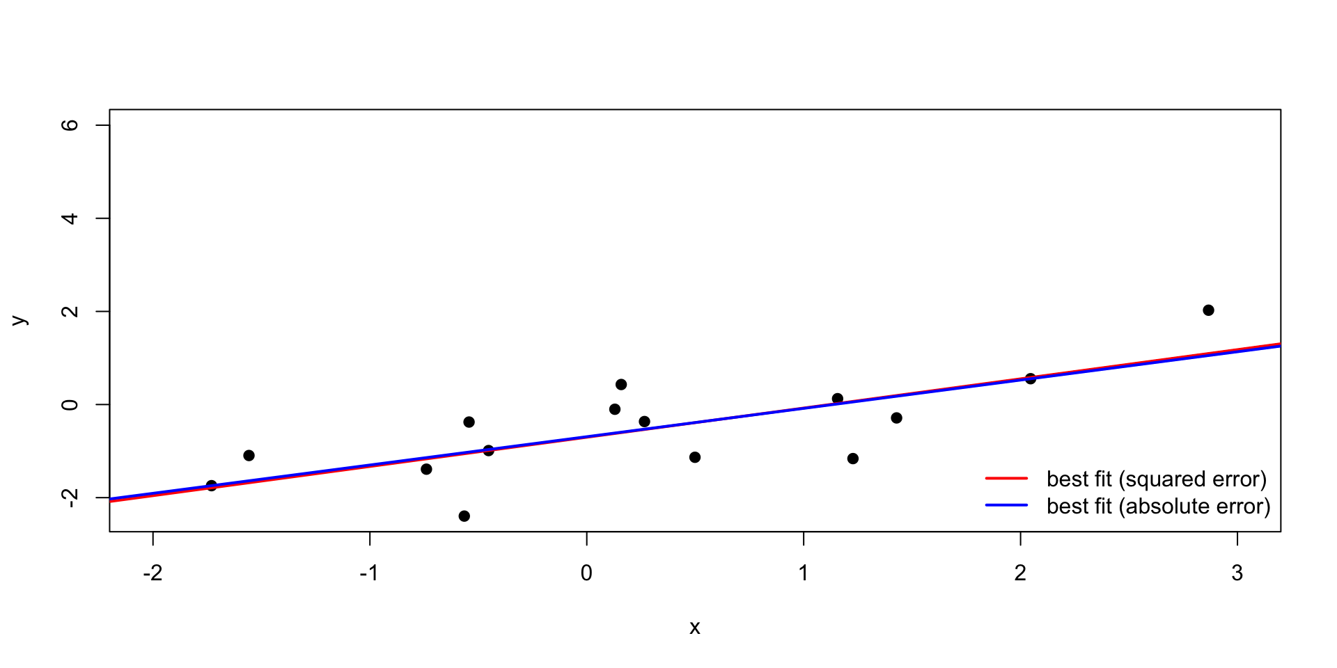
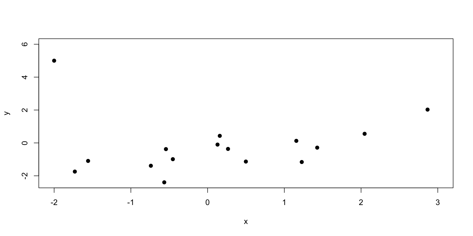
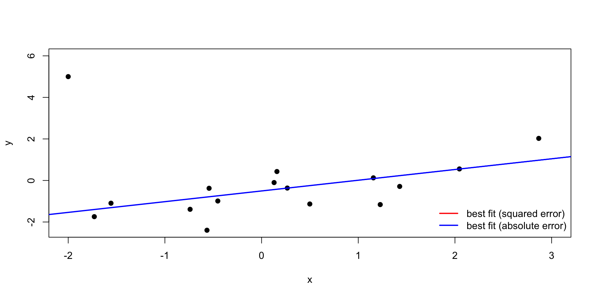
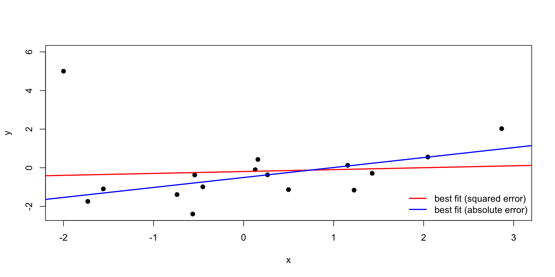
Squared error gives increasingly more weight to data points that are far away from the others; absolute error is more chill.

Toy dataset

Best fit line is basically the same either way

Best fit line is basically the same either way

Add an “outlier”

Blue doesn’t care

Red freaks out

Squared versus absolute error

• Minimizing absolute error instead of squared error is like using the median instead of the mean. It is “more robust” to outliers;
• These options are both “first class citizens;”
• But squared error is more common because it is more mathematically convenient, so that’s what we focus on.

R basics

Least squares line

movies_fit <- linear_reg() |>
  fit(audience ~ critics, data = movie_scores)

tidy(movies_fit)

# A tibble: 2 × 5
  term        estimate std.error statistic  p.value
  <chr>          <dbl>     <dbl>     <dbl>    <dbl>
1 (Intercept)   32.3      2.34        13.8 4.03e-28
2 critics        0.519    0.0345      15.0 2.70e-31

fit syntax

If you recall ggplot, it takes two arguments: a data frame and an aesthetic mapping that specifies what columns to use and how to use them. fit is similar. It takes two arguments: a data frame and a formula that species what variables to include in the model and how.

linear_reg() |>
  fit(y ~ x, df)

The statement y ~ x is called a formula in R. The variable name that appears to the left of the tilde (~) is treated as the response variable, and the variable(s!) to the right of the tilde are treated as explanatory.

Prediction

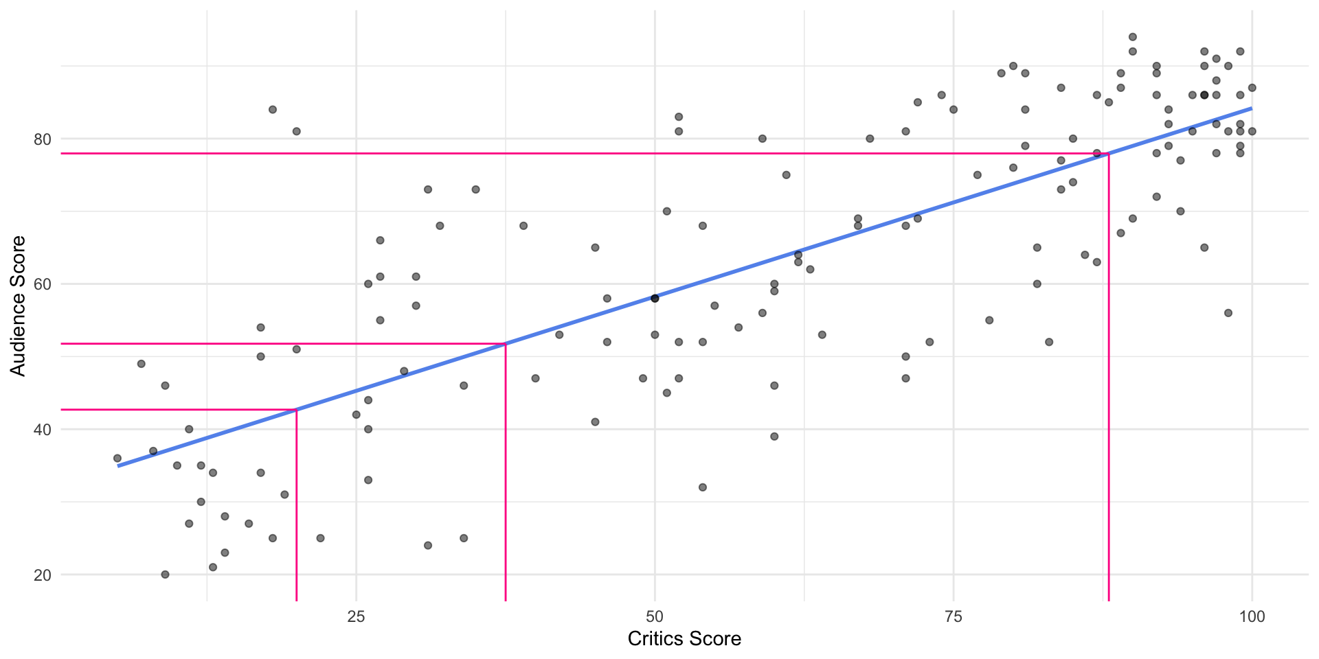
A new movie with a critics’ score of \(x = 20\) is released, and our model predicts that the audience score will be \(\widehat{y}\approx 42.69\), on average:

new_movie <- tibble(
  critics = c(20)
)

predict(movies_fit, 
        new_data = new_movie)

# A tibble: 1 × 1
  .pred
  <dbl>
1  42.7

Interpreting the slope and intercept

Correct

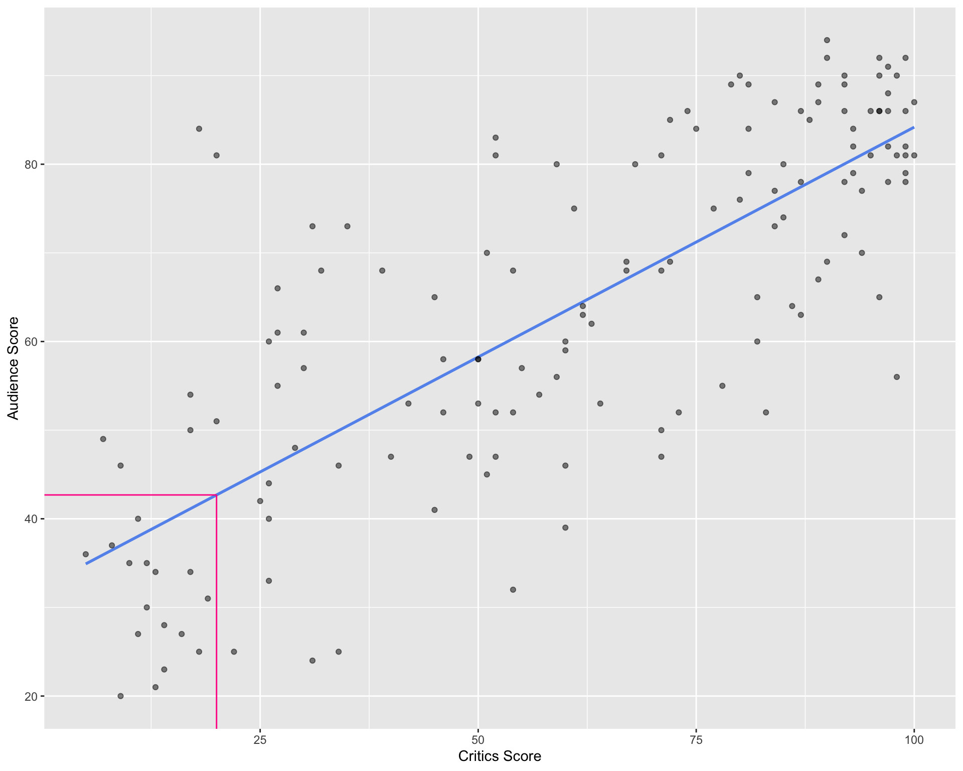
\[\widehat{\text{audience}} = 32.3 + 0.519 \times \text{critics}\]

• Slope: for every one point increase in the critics’ score, we expect the audience score to be higher by 0.519 points, on average;
• Intercept: for movies with a critics’ score of 0 points, we expect the audience score to be 32.3 points, on average.

The “we expect” and “on average” are a bit redundant, but let’s go belt and suspenders in this class.

Things to watch out for

When interpreting coefficient estimates in a regression:

• avoid causal-sounding language;
  • bad: “a one unit increase in x makes y go up by 0.519”
• don’t make guarantees;
  • bad: “if x = 0, then y will be 32.3”
• do be explicitly predictive;
  • good: “if x increases by one unit, we expect / predict that y will be higher by 0.519, on average.”

In general, our models give imperfect predictions about average behavior. The predictions are not guarantees, and the relationship may or may not be causal. Establishing that is an entire class in and of itself (causal inference).

Is the intercept meaningful?

✅ The intercept is meaningful in context of the data if

• the predictor can feasibly take values equal to / near zero, or
• the predictor has values near zero in the observed data

🛑 Otherwise, it might not be meaningful!

For example…

• It doesn’t make sense to predict the mpg of a car that weighs 0 pounds;
• It does make sense to predict the ice duration of a lake at 0 degree temp;
• It does make sense to predict audience score if the critics gave the movie a 0%.

A few FYIs

Properties of least squares regression

• The regression line always goes through the center of mass point (\(\bar{x}, \bar{y}\)) (ie. the coordinates corresponding to average \(X\) and average \(Y\)):

  • Why? Under LSR (least-squares regression), \(b_0 = \bar{y} - b_1~\bar{x}\); plugging in \(x =\bar{x}\) to the fitted eq, \(\widehat{y} = b_0 + b_1~\bar{x} = (\bar{y} - b_1~\bar{x}) + b_1~\bar{x} = \bar{y}\);

  • \(\Rightarrow \widehat{y} = \bar{y} \text{ when } x = \bar{x}\);

• Slope has the same sign as the correlation coefficient: \(b_1 = r \frac{s_Y}{s_X}\);

• Sum of the residuals is zero: \(\sum_{i = 1}^n \epsilon_i = 0\);

• Residuals and \(X\) values are uncorrelated.

First taste: goodness-of-fit

Goodness-of-fit

• Correlation is a number between -1 and 1 measuring the strength and direction of the linear association between two numerical variables (\(X\) and \(Y\));
• If you square it, you get \(R^2\) (“\(R\) squared”) or the coefficient of determination;
• This is a number between 0 and 1 measuring how well the linear model fits the data:
  • \(R^2=1\) means linear fit is perfect;
  • \(R^2=0\) means linear fit is perfectly wretched;
• Technically, \(R^2\) measures the fraction of the variation in the response \(Y\) explained by the model (more on this later).

Correlation and \(R^2\)

df |>
  summarize(
    r = cor(x, y)
  )

# A tibble: 1 × 1
      r
  <dbl>
1    -1

linear_reg() |>
  fit(y ~ x, df) |>
  glance() |>
  select(r.squared)

# A tibble: 1 × 1
  r.squared
      <dbl>
1         1

Correlation and \(R^2\)

df |>
  summarize(
    r = cor(x, y)
  )

# A tibble: 1 × 1
       r
   <dbl>
1 -0.935

linear_reg() |>
  fit(y ~ x, df) |>
  glance() |>
  select(r.squared)

# A tibble: 1 × 1
  r.squared
      <dbl>
1     0.875

Correlation and \(R^2\)

df |>
  summarize(
    r = cor(x, y)
  )

# A tibble: 1 × 1
       r
   <dbl>
1 -0.659

linear_reg() |>
  fit(y ~ x, df) |>
  glance() |>
  select(r.squared)

# A tibble: 1 × 1
  r.squared
      <dbl>
1     0.434

Correlation and \(R^2\)

df |>
  summarize(
    r = cor(x, y)
  )

# A tibble: 1 × 1
       r
   <dbl>
1 -0.335

linear_reg() |>
  fit(y ~ x, df) |>
  glance() |>
  select(r.squared)

# A tibble: 1 × 1
  r.squared
      <dbl>
1     0.112

Correlation and \(R^2\)

df |>
  summarize(
    r = cor(x, y)
  )

# A tibble: 1 × 1
       r
   <dbl>
1 -0.118

linear_reg() |>
  fit(y ~ x, df) |>
  glance() |>
  select(r.squared)

# A tibble: 1 × 1
  r.squared
      <dbl>
1    0.0140

Correlation and \(R^2\)

df |>
  summarize(
    r = cor(x, y)
  )

# A tibble: 1 × 1
      r
  <dbl>
1 0.117

linear_reg() |>
  fit(y ~ x, df) |>
  glance() |>
  select(r.squared)

# A tibble: 1 × 1
  r.squared
      <dbl>
1    0.0136

Correlation and \(R^2\)

df |>
  summarize(
    r = cor(x, y)
  )

# A tibble: 1 × 1
      r
  <dbl>
1 0.538

linear_reg() |>
  fit(y ~ x, df) |>
  glance() |>
  select(r.squared)

# A tibble: 1 × 1
  r.squared
      <dbl>
1     0.289

Correlation and \(R^2\)

df |>
  summarize(
    r = cor(x, y)
  )

# A tibble: 1 × 1
      r
  <dbl>
1 0.923

linear_reg() |>
  fit(y ~ x, df) |>
  glance() |>
  select(r.squared)

# A tibble: 1 × 1
  r.squared
      <dbl>
1     0.853

Correlation and \(R^2\)

df |>
  summarize(
    r = cor(x, y)
  )

# A tibble: 1 × 1
      r
  <dbl>
1     1

linear_reg() |>
  fit(y ~ x, df) |>
  glance() |>
  select(r.squared)

# A tibble: 1 × 1
  r.squared
      <dbl>
1         1

Recap: the anatomy of simple linear regression

Notation

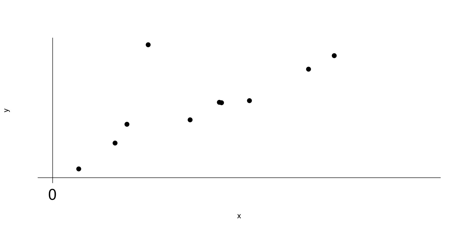
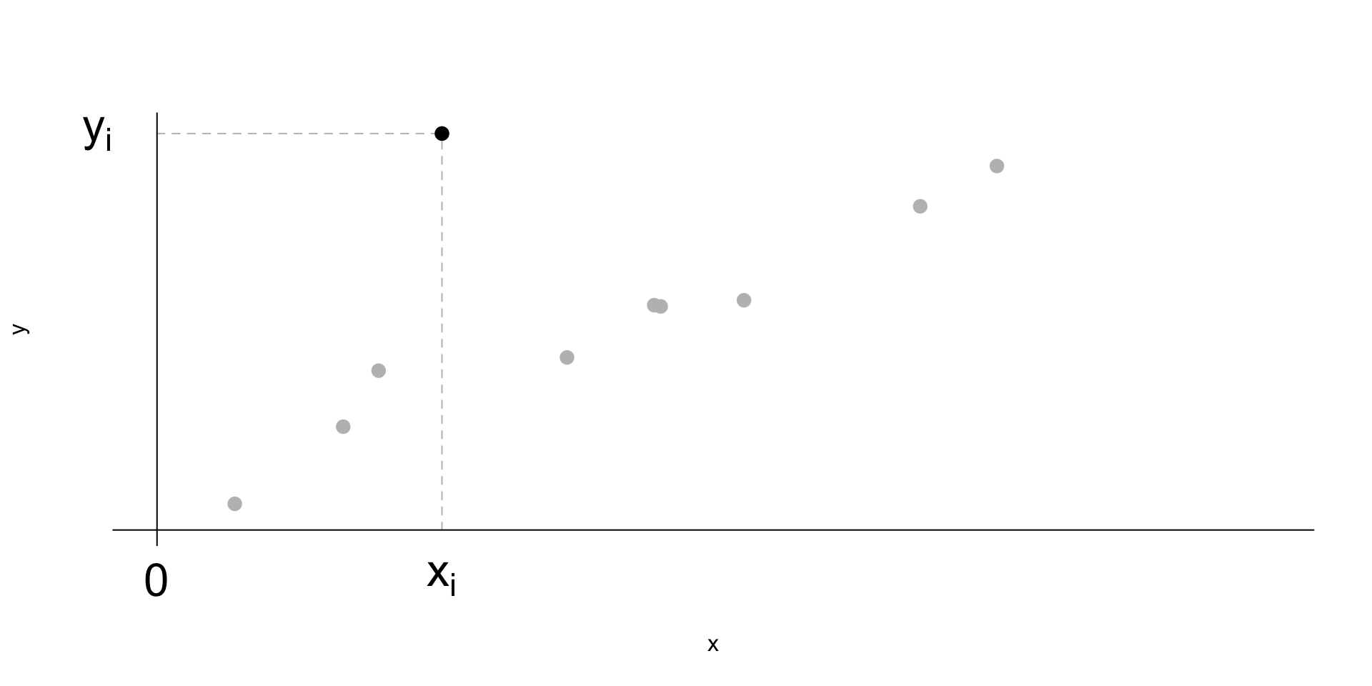
Imagine a data frame with \(n\) rows and 2 numerical columns

	x	y
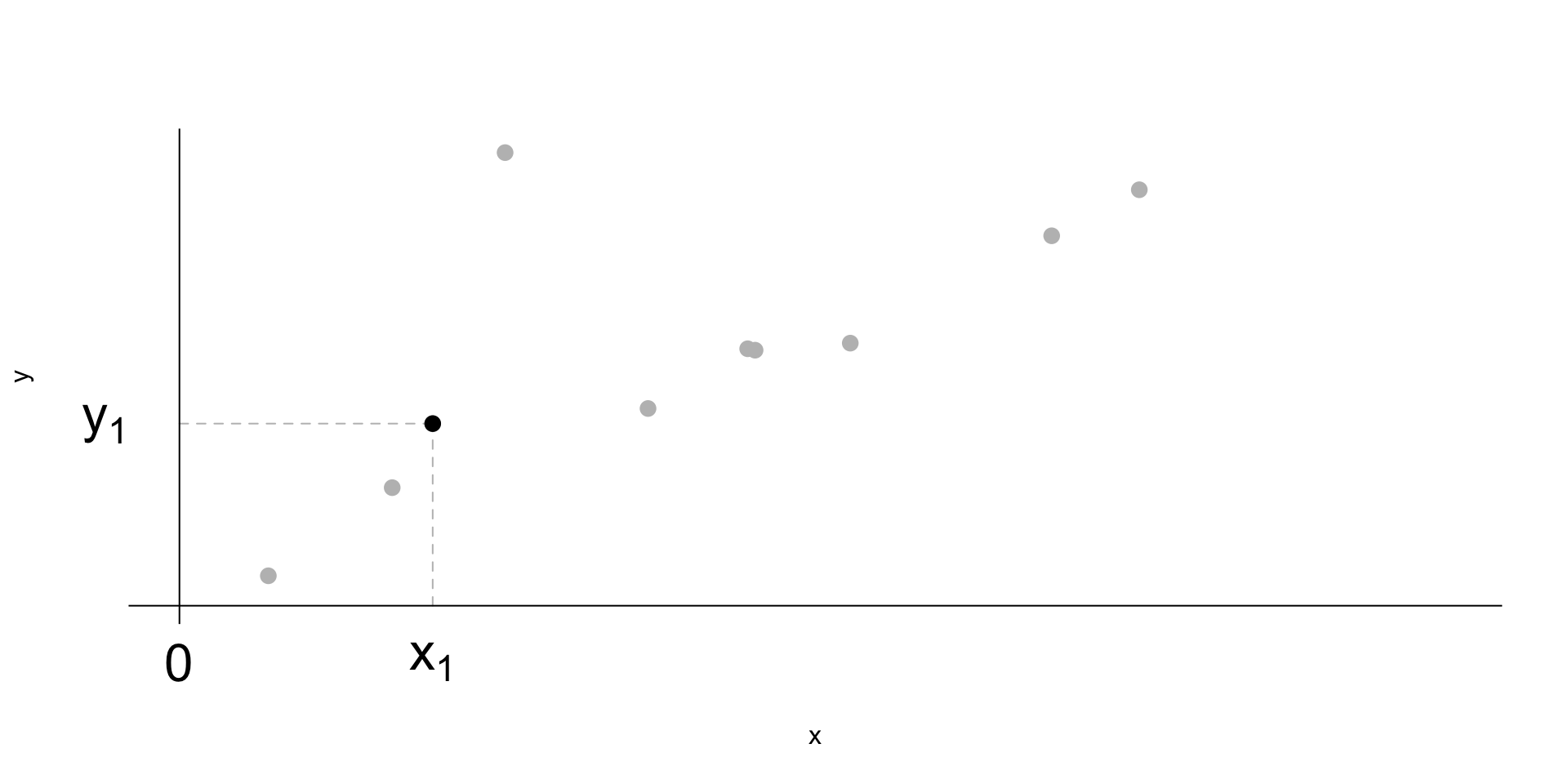
1	\(x_1\)	\(y_1\)
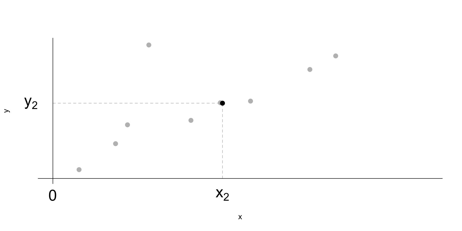
2	\(x_2\)	\(y_2\)
3	\(x_3\)	\(y_3\)
\(\vdots\)	\(\vdots\)	\(\vdots\)
\(i\)	\(x_i\)	\(y_i\)
\(\vdots\)	\(\vdots\)	\(\vdots\)
\(n-1\)	\(x_{n-1}\)	\(y_{n-1}\)
\(n\)	\(x_n\)	\(y_n\)

• We have \(n\) observations (ie. the sample size)

• \(i^{th}\) observation (\(i\) from \(1\) to \(n\)):

  • \(y_i\) : \(i^{th}\) outcome;

  • \(x_i\) : \(i^{th}\) explanatory variable;

  • \(\widehat{y_i}=b_0+b_1x_i\) : \(i^{th}\) predicted outcome;

  • \(e_i=y_i-\hat{y}_i\) : \(i^{th}\) residual.

The anatomy of simple linear regression

The data:

The anatomy of simple linear regression

The first row of the data frame:

The anatomy of simple linear regression

The second row of the data frame:

The anatomy of simple linear regression

The \(i\)th row:

The anatomy of simple linear regression

The line of best fit:

The anatomy of simple linear regression

The slope \(b_1=r\cdot s_Y/s_X\):

The anatomy of simple linear regression

The intercept \(b_0=\bar{y}-b_1\bar{x}\):

The anatomy of simple linear regression

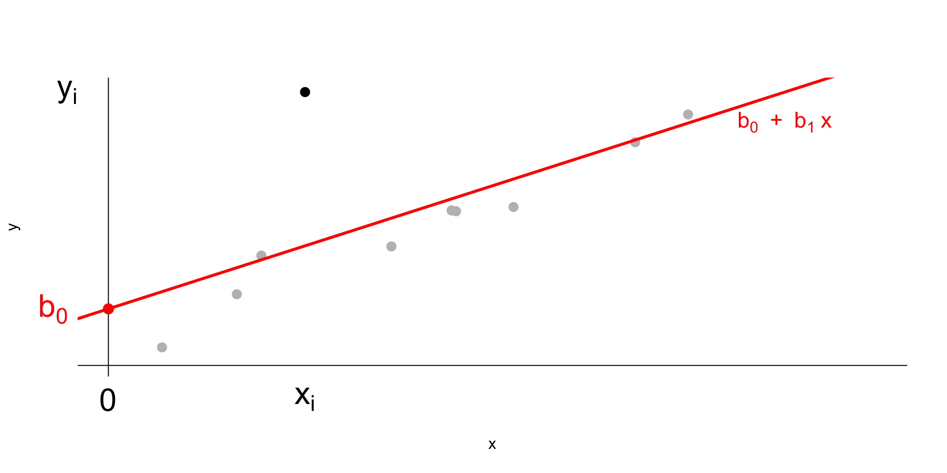
The line always passes through \((\bar{x},\,\bar{y})\):

The anatomy of simple linear regression

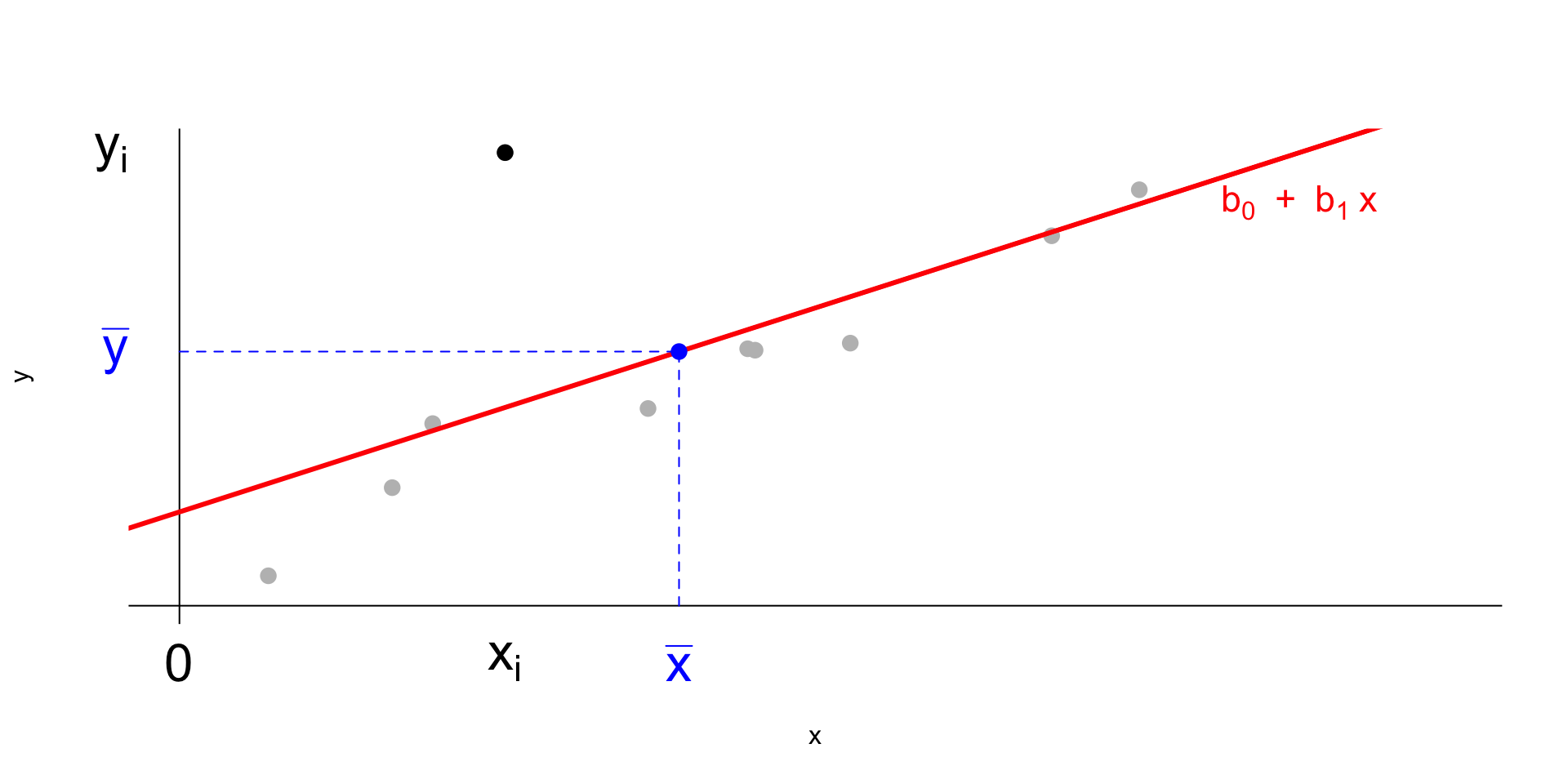
The prediction at \(x_i\):

The anatomy of simple linear regression

The residual: